Fig 1. Hele-Shaw flow past a circle

Experiment

Simulation

Theory #

Hele-Shaw flow #

Hele-Shaw flow is characterized as flow through the narrow gap between two parallel plates. The wall-contact induced viscous shear stresses lead to flow patterns that may be described as if the flow were ‘potential’. As the caption of this figure says, this may seem paradoxical: potential flows are those that are free of viscous stresses.

In the next two subsections we describe this effect mathematically. We start with the equations of viscosity dominated incompressible, creeping, flow (the Stokes equations), and show that they reduce to the potential flow equations for an inviscid fluid (the Darcy equations) in the case of fluid forced in between two parallel plates.

Stokes equations: from 3D to 2D #

When an incompressible fluid is characterized by a sufficiently low Reynolds number, the advective effects may be neglected and we retrieve the Stokes equations: $$ \begin{cases} \mu \Delta \mathbf{u} - \nabla p = \mathbf{0} \\ \nabla \cdot \mathbf{u} = 0 \end{cases} $$ where the time-derivative terms is dropped as we assumed that steady state is reached.

The “flattened” appearance of the flow in a narrow slit may lead one to naïvely conclude that Hele-Shaw flow should be modeled as a 2D Stokes goverened system. This is quite untrue: it is precisely in that third dimension that high velocity gradients occur, leading to high viscous drag forces. We thus ought to start our analysis from the three-dimensional Stokes equations: $$ \begin{cases} \mu ( \frac{\partial^2}{\partial x^2} u_x + \frac{\partial^2}{\partial y^2} u_x + \frac{\partial^2}{\partial z^2} u_x ) - \frac{\partial}{\partial x} p = 0 \\ \mu ( \frac{\partial^2}{\partial x^2} u_y + \frac{\partial^2}{\partial y^2} u_y + \frac{\partial^2}{\partial z^2} u_y ) - \frac{\partial}{\partial y} p = 0 \\ \mu ( \frac{\partial^2}{\partial x^2} u_z + \frac{\partial^2}{\partial y^2} u_z + \frac{\partial^2}{\partial z^2} u_z ) - \frac{\partial}{\partial z} p = 0 \\ \frac{\partial}{\partial x}u_x + \frac{\partial}{\partial y}u_y + \frac{\partial}{\partial z} u_z = 0 \end{cases} $$

Focusing first on the velocity dependence on the third dimension, we note that such wall-bounded channel flow has its own name: Poiseuille flow. The well-known corresponding velocity profile is a quadratic function that is zero at the two walls, and achieves its maximum at the center. Schematically, the velocity profile through the gap width looks like:

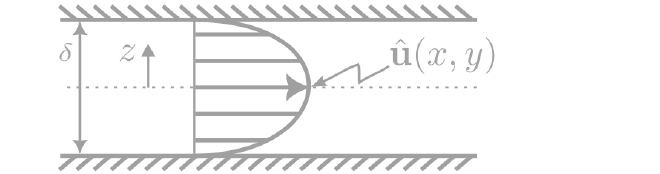
Making use of this knowlegde, we can write our full three-dimensional velocity field \(\mathbf{u} = \mathbf{u}(x,y,z)\) just in terms the two-dimensional center velocity \(\hat{\mathbf{u}} = (\hat{u}_x , \hat{u}_y , 0 )^\text{T} = \hat{\mathbf{u}}(x,y) \): $$ \mathbf{u}(x,y,z) = (1 - \frac{2}{\delta} z ) \, ( 1 + \frac{2}{\delta} z ) \, \hat{\mathbf{u}}(x,y) \,, $$ where \( \delta \) is the width of the gap. By construction, this assumed flow profile satisfies the no-slip boundary conditions at the two parallel plates: \( \mathbf{u}(x,y,\delta/2) = \mathbf{u}(x,y,-\delta/2) = \mathbf{0} \), and simply equals the center velocity at the midpoint: \( \mathbf{u}(x,y,0) = \hat{\mathbf{u}}(x,y) \).

When this assumed velocity profile is substituted into the three-dimensional Stokes equations, they produce: $$ \begin{cases} \mu ( \frac{\partial^2}{\partial x^2} \hat{u}_x + \frac{\partial^2}{\partial y^2} \hat{u}_x - \frac{8}{\delta^2} \hat{u}_x ) - \frac{\partial}{\partial x} p = 0 \\ \mu ( \frac{\partial^2}{\partial x^2} \hat{u}_y + \frac{\partial^2}{\partial y^2} \hat{u}_y - \frac{8}{\delta^2} \hat{u}_y ) - \frac{\partial}{\partial y} p = 0 \\ \frac{\partial}{\partial z} p = 0 \\ \frac{\partial}{\partial x}\hat{u}_x + \frac{\partial}{\partial y}\hat{u}_y = 0 \end{cases} $$ or, in vector notation: $$ \begin{cases} \mu \Delta \hat{\mathbf{u}} - \nabla \hat{p} = \frac{8 \mu}{\delta^2} \hat{\mathbf{u}} \\ \nabla \cdot \hat{\mathbf{u}} = 0 \end{cases} $$ where \( \hat{p} = \hat{p}(x,y) \), and the Laplace and gradient operators can now be understood as two-dimensional differential operators.

Darcy equations #

As may be observed from this dimensionally-reduced Stokes-like equation, the effect of the viscous wall-shear stress manifests itself as a drag force that scales linearly with the center velocity. In its current form, the equations are called the Darcy-Brinkman equations. However, if \( \mu \Delta \hat{\mathbf{u}} \ll \frac{8 \mu}{\delta^2} \hat{\mathbf{u}} \), as would be the case when \(\delta\) is much smaller than the other geometric features, then the remaining viscous stress may be neglected, and we find: $$ \begin{cases} \hat{\mathbf{u}} = - \frac{\delta^2}{8 \mu} \nabla \hat{p} \\ \nabla \cdot \hat{\mathbf{u}} = 0 \end{cases} $$ which are the Darcy equations.

The Darcy and Stokes equations leads to quite different solution fields. This can be observed in the figures below, for which the same streamline inflow locations have been chosen. In case of Stokes flow, the effect of the obstructing cylinder is noticible much further upstream.

Stokes

Darcy

Simulation #

Finite element formulation #

The focus of the current post is on the Hele-Shaw theory section. As such, the section of the mathematics behind the finite element approximation is kept relatively short, and may seem overly concise to the uninitiated. Other posts will focus more on this aspect.

To obtain a finite element approximation, we require a weak formulation of the partial differential equation at hand. The Sokes and Darcy equations are both systems of differential equations. In weak form, these lead to so-called mixed formulations. For the Darcy equations, we obtain: $$ \text{Find } (\hat{\mathbf{u}}, \hat{p} ) \in \mathbf{H}_{h}(\text{div}) \times L^2 \text{ s.t.}: \qquad\qquad\quad\qquad\quad\qquad\quad\\ \begin{cases} \int \big( \frac{8 \mu}{\delta^2} \hat{\mathbf{u}} \cdot \mathbf{v} - \hat{p} \, \nabla \cdot \mathbf{v} \big) \text{d}S = - \int g \, \mathbf{v}\cdot\mathbf{n} \, \text{d}L \quad \forall\, \mathbf{v} \in \mathbf{H}_0 (\text{div}) \\ \int q\,\nabla \cdot \hat{\mathbf{u}} \text{d}S = 0 \qquad\qquad\qquad\qquad\qquad\quad\,\,\, \forall\, q \in L^2 \end{cases} $$ where \( L^2 \) is the space of square integrable functions and \( \mathbf{H}(\text{div}) \) is the space of vector-valued functions whose divergence’s are functions in \( L^2 \). Members of \( \mathbf{H}(\text{div}) \) permit evaluation of their normal component on domain boundaries, whereby \( \hat{\mathbf{u}}\cdot\mathbf{n} = h \) represents an essential condition which is thus imposed on all functions in the space \( \mathbf{H}_{h} (\text{div}) \) (c.q. \( \mathbf{v}\cdot\mathbf{n} = 0 \) on \( \mathbf{H}_{0} (\text{div}) \)). The natural condition is the imposed pressure \( \hat{p}=g \), which is already substituted in the right-hand-side integral in the above equation. The chosen values for all boundary conditions are illustrated in the figure below.

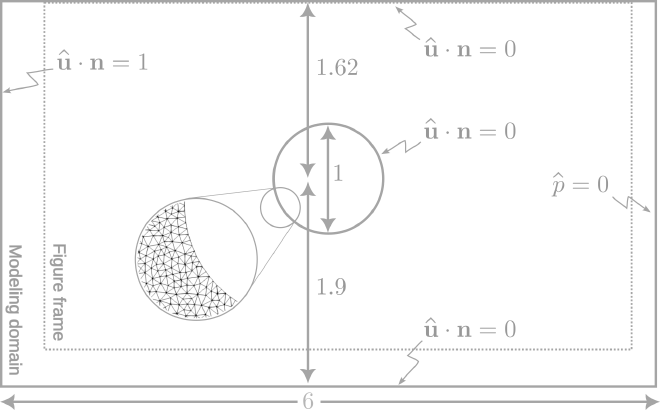
The bottom of the computational domain is chosen slightly larger than the figure frame, as the streamlines in the original figure slightly curve out of the frame. This figure also shows the relative dimensions used for the computational domain. Units are purposely left out: the qualitative nature of the solutionfield (i.e., the streamslines) is not affected by the scale of the domain, nor by the magnitude of the inflow, or even by the value of the effective permeability \( \frac{8 \mu}{\delta^2} \).

While devising a finite element approximation of the above weak formulation, one must take care to choose an appropriate pair of discrete function spaces. Not every choice of vector-valued velocity and scalar-valued pressure finite element spaces is “stable” and produces accurate results, or even produces a solveable system of equations. Typical compatible spaces for the Darcy equations, are a \( P \)-th order Brezzi-Douglas-Marini (BDM) space for the velocity and a \( ( P-1 ) \)-th discontinuous Galerkin (DG) space for pressure, or \( P \)-th order Raviart-Thomas (RT) space paired with a \( ( P-1 ) \)-th order DG space. In the following implementation, we make use of BDM elements. The mesh size used is illustrated in the figure above.

Code implementation #

This simulation is performed with the finite element method, with the library FEniCS. The following code outputs the required data:

from dolfin import *
from mshr import *

# Physical parameters
D = 1
L = 6
Ht = 1.62 # height till top
Hb = 1.9 # height till bottom

# Numerical parameters
resolution = 120

# Create mesh
domain = Rectangle(Point(-L/2,-Hb),Point(L/2,Ht)) - Circle(Point(0,0), D/2)
mesh = generate_mesh(domain, resolution)

# Create finite element spaces
BDM = FiniteElement("BDM", mesh.ufl_cell(), 1)
DG  = FiniteElement("DG", mesh.ufl_cell(), 0)
V = FunctionSpace(mesh, BDM * DG)

# Define test, trial and solution function
u, p = TrialFunctions(V)
v, q = TestFunctions(V)
u_sol = Function(V)

# Define boundary conditions
def boundary_noflow(x):
    return x[1] < -Hb+DOLFIN_EPS or x[1] > Ht - DOLFIN_EPS \
        or x[0]**2+x[1]**2 < (D/2)**2+DOLFIN_EPS
def boundary_inflow(x):
    return x[0] < -L/2+DOLFIN_EPS
bcs = [DirichletBC(V.sub(0), Constant((0,0)), boundary_noflow),\
      DirichletBC(V.sub(0), Constant((1,0)), boundary_inflow),]

# Weak formulation
a = (dot(u,v) + div(v)*p + div(u)*q)*dx
Lrhs = - Constant(0)*q*dx

# Solve and export
solve(a == Lrhs, u_sol, bcs)
(u,p) = u_sol.split()
u.rename('u','u')
File("sol.pvd") << u

Visualization #

Visualization is performed in Paraview, with the streamline and tube filters. The seeds of the streamlines are manually placed at the correct inflow points. The tube filter permits a variable tube width, as specified by a minimum value, a maximum scaling w.r.t that minimum value, and a scalar-field between whose minimal and maximal values is interpolated. For the latter, we specify a simple \(\frac{1}{\sqrt{|\mathbf{u}|}}\) function, representing the streching and broadening of the paint streak with increasing resp. decreasing flow velocity. Below follow screenshots of the visualization settings, and some further visualizations of the qualitative behavior of the solution.