Fig 34. Boundary-layer separation on an inclined airfoil

Experiment

Simulation

“When the NACA 64A015 airfoil of figure 23 is raised to 5\(\degree\) incidence the laminar boundary layer separates from the rear half of the upper surface. The flow remains attached to the lower surface, from which it leaves tangentially at the trailing edge. Streamlines are shown by colored fluid filaments in water.” ONERA photograph, Werlé 1974

Boundary layer theory #

In the web post from Figure 23 boundary layer theory was introduced and applied to an airfoil without separation. Here, we revisit the same airfoil geometry, now at a higher incidence, where we explore how and why separation occurs.

Boundary-layer flow separation #

As established, a positive pressure gradient slows down the fluid near the wall. When the gradient becomes sufficiently strong, the velocity close to the wall may reverse. This reversal can only occur under a positive pressure gradient because the free-stream flow continues in the original direction. This implies that the velocity profile must develop an inflection point, which is a characteristic that only happens with positive pressure gradients.

A separation point can then be defined as the location where the forward and reversed flows meet. At the separation point, the streamwise velocity vanishes, because the flow becomes purely vertical due to incompressibility.

Pressure gradient over airfoil #

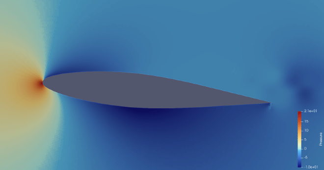
Below the pressure around the airfoil from figure 34 is shown. The pressure distribution maintains a similar trend as in figure 23: at the leading edge there is a negative pressure gradient, but it is not present down to the middle of the airfoil, instead, it transitions to a positive gradient much faster. In the middle of the airfoil, the pressure gradient is already positive. The pressure gradients are also significantly stronger than in figure 23.

Velocity profiles over airfoil #

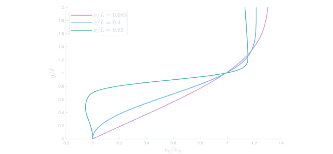
The increased positive gradient strongly influences the boundary layer behaviour, as seen in the tangential velocity profiles below. At \(x/L = 0.083\) the flow is still attached and looks similar to the Blasius solution. At \(x/L = 0.4\) the profile develops an inflection point, indicating that the flow is decelerating and the positive pressure gradient is affecting the flow. Finally, at \(x/L=0.83\), the flow separation is evident, since the near-wall velocity has reversed.

Separation leads to increased pressure drag and reduced lift, significantly lowering the airfoil’s aerodynamic efficiency. Therefore, such behaviour is typically avoided when designing an airfoil, unless the separated region can be controlled or predicted.

Concluding remarks #

Boundary-layer theory explains how the near-wall velocity profiles are affected by pressure gradients, and why flow may remain attached or separate. In this post, we applied the theory to the case of separated flow, and observed that the CFD results behave as expected: negative gradients yield steeper velocity profiles, while positive gradients produce inflection points and eventually flow reversal near the wall.

Simulation #

To replicate the original figure by H. Werlé in the ONERA water tunnel, the simulation was carried out using Star-CCM+.

Geometry #

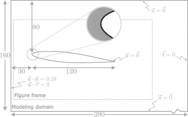
The same airfoil and water tunnel were used for both figure 23 and figure 34. However, since this figure corresponds to a different Reynolds number, the inlet velocity must be recalculated. In the original source, the Reynolds number is given as \(Re_L = 24000\) [1]. Assuming water at \(25\degree C\) we get:

$$ \begin{gather*} Re_L = \frac{\rho v_{\infty} L}{\nu} = 24000 \\ v_{\infty} = \frac{24000 \cdot 8.8871\cdot{10}^{-4}}{997.561 \cdot 0.12} = 0.18\ m/s \end{gather*} $$

Meshing #

A 2D mesh was used in this case, as the 3D mesh failed to produce accurate results. The base size was set to \(5\cdot 10^{-4}\ m\) and 45 prism layers were used at a height of \(3\cdot 10^{-4} m\), resulting in a total of 392295 cells. The top and bottom of the domain were set to no-slip walls to simulate the walls of the water tunnel.

The physics models and visualisation steps were identical to those for Figure 23.

References #

[1] Werlé, H.. Le Tunnel hydrodynamique au service de la recherche aérospatiale. O.N.E.R.A 1974