Fig 35. Leading-edge separation on a plate with laminar reattachment
Table of Content
Air bubbles in water show the turbulent flow field and laminar reattachment on an inclined plate at Reynolds number \(Re = 10000\). At \(2.5^{\circ}\) inclination relative to the oncoming flow, the flow briefly separates from the upper surface at the leading edge before it reattaches to the inclined plate. The separation region creates a recirculating turbulent boundary layer. For comparison, a transient simulation was created in Simcenter StarCCM+ using the SST turbulence model. Photograph by ONERA photograph, Werlé 1974
Turbulence transition #
The flow field over a \(2.5^{\circ}\) inclined plate shows a large transition region between laminar and turbulent flow. This is an ideal case for putting turbulence models to the test. For the comparison figure between the experiment picture and the simulation visualization, the SST turbulence model was used. However, this simulation was also run with the k-epsilon and k-omega turbulence models, with a model comparison given below. A detailed overview about RANS turbulence models is given in Figure 47 and all of the theory referring to k-epsilon, k-omega and SST turbulence models can be found there.
Simulation #
All of the simulations of the inclined plate experiment were carried out in Simcenter StarCCM+ using the k-epsilon, k-omega and SST turbulence models. The differences in results of each of the turbulence models will be discussed in the ‘Visualization’ section of this post, since the differences become apparent during post-processing.
Computational domain #
As with all replications of the figures from the book, the computational domain, boundary conditions and finite volume mesh are created with the highest possible fidelity to the information available in the caption of the original picture. In this case it is known that the flow field is visualized with air bubbles in water and that the flow is characterized by the Reynolds number \(Re = 10000\) based on the length of the plate. The length of the plate can be calculated to be \(0.1\ m\) and the inlet velocity to be \(0.1\ m/s\) with the incidence angle set to \(2.5^{\circ}\). The walls of the domain have a no-slip condition applied to them, the inlet is specified as a velocity inlet and the outlet as a pressure outlet. Since this experiment closely resembles the setup of an airfoil simulation, the domain size was set accordingly an can be seen in the figure below. The beveled edges were recreated as close as possible and the plate thickness was set to \(2\)% of the length, as is stated in the caption of the original figure.
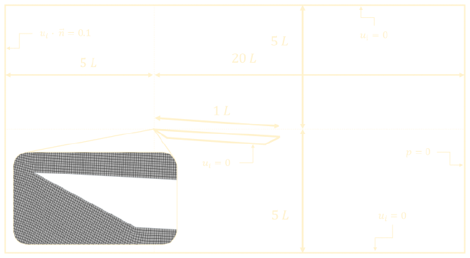
The base size of the quadrilateral FVM mesh is set to \(0.001\ m\). To save on computational expenses, this base size is only applied in the region near the inclined plate. The custom mesh controls available in StarCCM+ are used to coarsen the mesh in the far-field parts of the domain. The domain walls have an element size of \(0.3\ m\) (\(30000\)% of base size) and the global growth rate is set to \(1.1\). On top of this, further refinement is applied in the boundary layer region of the plate. Namely the element size in this region is set to \(10\)% of the base size. The total cell count of this FVM mesh is \(102617\). Visualizations of this mesh can be seen below.
StarCCM+ setup #
The simulation setup in StarCCM+ is the exact same as mentioned in this post about flow over a circular cylinder. More details and information about the simulation setup can be found there. What’s important to note is that three simulations were run in a transient environment, one using the low Reynolds number k-epsilon model, one using Wilcox’s (2008) k-omega model and a last one using Menter’s SST model.
Visualization #
Post processing and visualization in done in
Paraview. Compared to the visualizations discussed in
this post about flow over a circular cylinder and
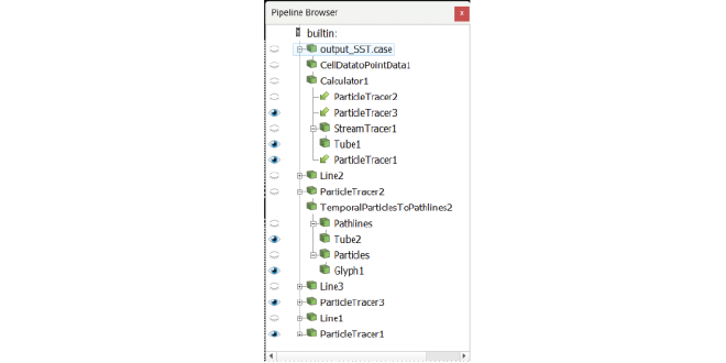
this post about flow over a large angle plate, the \(2.5^{\circ}\) inclined plate has less chaotic and small scale turbulent phenomena. Therefore this visualization is mostly based on the streamlines of the flow field and allows for a better quantitative comparison between different turbulent models. As with other visualizations, the output data must be transformed from cell data to point data using the CellDatatoPointData filter in ParaView. From here, the velocity vector can be computed with the Calculator filter, adding the X and Y velocities with their respective unit vectors. The StreamTracer filter can now be applied to the velocity field and can be visualized with the Tube filter on top of it. However, the stream lines don’t show the recirculating bubble boundary layer at the leading edge of the plate, thus some particles can be injected here. For this, the Line source is used, to which the ParticleTracer and TemporalParticlestoPathlines filter can be added on top of. The full ParaView pipeline is shown below.
The final visualization can be seen in the slider at the top of the page for the comparison between the closest result of the numerical simulation and the actual experiment picture. For the final visualizations, the timesteps were matched to that of SST model with the most accurate visualization compared to the original figure. It should be noted that the best matching timestep is not in the ‘steady state’ of the transient simulation. All of the simulations show a more elongated separation bubble at the leading edge of the plate after a long enough physical time period, which can be assumed to show the steady state. There could be multiple reasons for this, the most probable being a slightly inaccurate simulation geometry model compared to the plate used in the experiment. There are no specific details about the beveled edges of the real plate, so these were simply modeled as close as possible to the actual plate. The visualizations of the all of the turbulence model results can be seen in the slider figures below.
As can be seen from the second slider, the difference in flow field prediction between the k-omega and SST model are barely noticeable. This is to be expected, since in the SST model, the blending function activated the k-omega model in the near wall region, thus both models should predict a similar flow field close to the wall boundary. However, there is a noticeable difference between the k-epsilon and k-omega model when comparing the height of the recirculating separation bubble at the leading edge of the plate.
Turbulence model comparison #
To further highlight the difference in boundary layer height prediction between the two k-omega models (k-omega and SST) and k-epsilon model, some post processing filters can be applied to the velocity field of the simulation outputs at equal timesteps. First, one can add a grid to the background of the graphics window in order to quantify the actual boundary layer height. However, the grid (or the data) must be rotated 2.5 degrees using the Transform filter in order to turn the plate horizontally and be able to measure the boundary layer height normal to the plate. Then, a Contour filter can be added with a customized value range for different definitions of the boundary layer thickness. In general, the boundary layer thickness is defined as the height \(\delta\) where
$$
u(x, \delta_{99}) = 0.99 \ u_{\infty}
$$
with \(\delta_{99}\) the normal distance to the plate surface where the velocity magnitude is \(99\)% that of the freestream velocity. To better highlight the boundary layer height in these simulations, multiple different velocity definitions of the boundary layer thickness are taken. Namely the normal distance to \(50\)%, \(60\)%, \(70\)%, \(80\)%, \(90\)% and \(95\)% of the freestream velocity. The result of these post processing steps and the difference between the boundary layer prediction of the k-epsilon and k-omega models can be seen in the slider below.
Although the simulation results can only be compared to the picture of the experiment results and not actual data, the SST and k-omega turbulence model seem to be the most accurate, as can be seen in the slider figure at the very top of the page. If the k-omega and SST model are taken as reference, the slider figure just above shows that the k-epsilon model under-predicts the boundary layer height. The graphs above actually show that at \(15\)% of the plate length (\(x=0.015\ m\)), the k-epsilon model predicts a \(\delta_{70}\) boundary layer height where the k-omega and SST models predict a \(\delta_{50}\) boundary layer height. As for the \(\delta_{95}\) boundary layer height, the k-epsilon model predicts a \(10\)% lower boundary layer height than the two k-omega models.
Knowing how these models behave, this behaviour is to be expected. As mentioned in the ‘Theory’ section in this post, the low Reynolds number k-epsilon model uses damping functions on the coefficients in the model for the energy dissipation rate \(\epsilon\). Although these damping functions greatly increase the near-wall flow prediction compared to the standard k-epsilon model, they are empirical functions and are simply not as accurate as a direct modelling approach found in the k-omega and SST model. These models are based on the specific energy dissipation rate \(\omega = \frac{\epsilon}{k}\), which is the energy dissipation rate per unit kinetic turbulent energy and thus do not need empirical damping functions on the model coefficients.
Another turbulence model comparison with an almost identical simulation and experiment setup to this one can be found on this page. This post also contains more information about the low Reynolds number k-epsilon model.