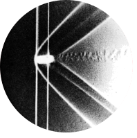
Fig 23. Symmetric plane flow past an airfoil

Experiment

Simulation

Boundary layer theory #

This post and the web post for figure 34 both feature the same NACA airfoil, but due to different Reynolds numbers and angles of attack, they show two very different results. In the current figure, the flow is laminar and remains attached, but for figure 34 the flow separates. To understand the physical mechanisms behind this change, we turn to boundary layer theory. By applying this to a flat plate first and then to an airfoil, we can explain when and why separation occurs, and assess whether our CFD results capture this behaviour accurately.

Boundary layer definition #

At large Reynolds numbers, the effects of viscosity are confined to a small region near a wall, known as the boundary layer [1]. In this layer, the velocity transitions from zero at the surface (due to the no-slip boundary condition) to the free-stream velocity just outside it. We will show that, despite its small size, the boundary layer strongly influences the overall flow behaviour.

Boundary layer over a flat plate #

To understand the behaviour of boundary layers, we begin with a simplified case: laminar flow over a flat plate with parallel inflow. In contrast to curved geometries such as airfoils, a flat plate allows for several simplifications and assumptions, whilst still giving us insight into the velocity profiles, boundary layer thickness and effects of pressure gradients.

To get the final equations for flow over a flat plate, we start with the Navier-Stokes equations, of which a derivation can be found in the post for figure 42. For a steady case, with an incompressible, Newtonian fluid these equations are given by: $$ \begin{gather*} \rho (\mathbf{u} \cdot \nabla)\mathbf{u} = -\nabla p + \mu \nabla^2 \mathbf{u} \\ \nabla \cdot \mathbf{u} = 0 \end{gather*} $$ where \(\rho\) is the fluid density, \(\mu\) is the dynamic viscosity, \(p\) is the pressure \(\nu = \mu/\rho\) is the kinematic viscosity, and \(\mathbf{u}\) is the velocity vector \(\mathbf{u} = \begin{bmatrix} v_x \\ v_y\\ v_z \end{bmatrix}\).

Now, we assume the plate to be infinitely deep, so that we can reduce 3D reality to a 2D representation. We also divide everything in the momentum equation by \(\rho\): $$ \begin{gather*} v_x\frac{\partial v_x}{\partial x} + v_y\frac{\partial v_x}{\partial y} = - \frac{1}{\rho}\frac{\partial p}{\partial x} + \nu\left(\frac{\partial^2 v_x}{\partial x^2} + \frac{\partial^2 v_x}{\partial y^2}\right)\\ v_x\frac{\partial v_y}{\partial x} + v_y\frac{\partial v_y}{\partial y} = - \frac{1}{\rho}\frac{\partial p}{\partial y} + \nu \left(\frac{\partial^2 v_y}{\partial x^2} + \frac{\partial^2 v_y}{\partial y^2}\right)\\ \frac{\partial v_x}{\partial x} + \frac{\partial v_y}{\partial y} = 0 \\ \end{gather*} $$

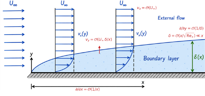
To see which of these terms matter inside the boundary layer, we estimate their orders of magnitude. Streamwise changes occur over the distance \(x\) from the leading edge, whereas wall-normal changes occur over the much smaller boundary layer thickness \(\delta\), so \(\frac{\partial}{\partial x} = \mathcal{O}\left(\frac{1}{x}\right)\) and \(\frac{\partial}{\partial y} = \mathcal{O}\left(\frac{1}{\delta}\right)\). The x-component velocity ranges from zero at the plate to the free-stream velocity \(U\) away from the plate, so \(v_x = \mathcal{O}(U)\).

The mass balance (continuity) equation states \(\frac{\partial v_x}{\partial x} = - \frac{\partial v_y}{\partial y}\). For both sides of the equation to balance given the above scalings requires \(v_y = \mathcal{O}\left(U\frac{\delta}{x}\right)\).

In the \(x\)-momentum equation, both convective terms are thus \(\mathcal{O}(U^2/x)\), while of the viscous terms only \(\nu \frac{\partial^2 v_x}{\partial y^2} = \mathcal{O}(\nu U/\delta^2)\) remains, since \(\nu \frac{\partial^2 v_x}{\partial x^2}\) is a factor \((\delta/x)^2\) smaller. Inside the boundary layer, inertia and viscosity must balance at leading order, which fixes its thickness: $$ \begin{gather*} \frac{U^2}{x} \sim \frac{\nu U}{\delta^2} \quad \Rightarrow \quad \delta \sim \sqrt{\frac{\nu x}{U}} = \frac{x}{\sqrt{Re_x}}, \qquad Re_x = \frac{U x}{\nu} \end{gather*} $$

So at high Reynolds numbers indeed \(\delta \ll x\). Applying the same estimates to the \(y\)-momentum equation, all inertial and viscous terms are \(\mathcal{O}(U^2\delta/x^2)\), so the pressure varies across the boundary layer by only \(\mathcal{O}(\rho U^2 \delta^2/x^2)\). To leading order \(\partial p/\partial y = 0\): the pressure is imposed on the boundary layer by the outer flow. This leaves the boundary layer equations:

$$ \begin{gather*} v_x\frac{\partial v_x}{\partial x} + v_y\frac{\partial v_x}{\partial y} = - \frac{1}{\rho}\frac{\partial p}{\partial x} + \nu \frac{\partial^2 v_x}{\partial y^2}\\ 0= - \frac{1}{\rho}\frac{\partial p}{\partial y}\\ \frac{\partial v_x}{\partial x} + \frac{\partial v_y}{\partial y} = 0 \\ \end{gather*} $$

We consider two different cases:

• One with a constant free stream velocity \(U = v_{\infty}\). As a result, the free stream pressure is also constant, \(\frac{dp}{dx} = 0\). Deriving the boundary layer profile for this case is known as the Blasius solution.
• And another with a free stream pressure gradient, which is equivalent to flow over a wedge (see figure below). This is the Falkner-Skan solution, where the pressure gradient exists due to variations in the free-stream velocity \(U = v_\infty x^{\frac{\beta}{2-\beta}} = v_\infty x^m\) [2], as explained via Bernoulli’s principle:

$$ \begin{gather*} \frac{1}{2}U^2 + \frac{p}{\rho} = constant \to -\frac{1}{\rho} \frac{\partial p}{\partial x} = U\frac{\partial U}{\partial x} \end{gather*} $$

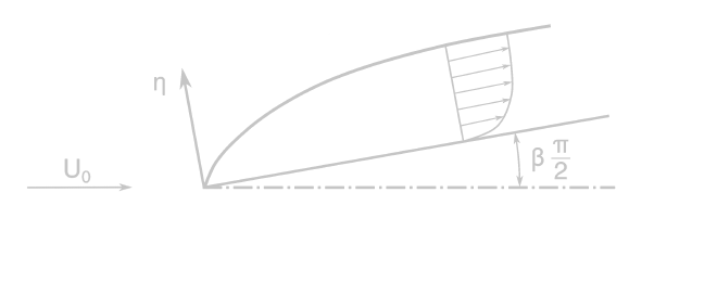
Here, \(\beta\) determines the streamwise pressure behaviour. \(\beta = 0\) corresponds to the flat plate case, leading to the Blasius solution. Negative \(\beta\) corresponds to a positive pressure gradient and positive \(\beta\) to a negative pressure gradient. In the steps below, we highlight the occurrences of \(\beta \), and thus the deviation from Blasius boundary-layer theory, in magenta.

The key step is a self-similarity ansatz: the velocity profiles at different \(x\) are assumed to have the same shape once the wall-normal coordinate is scaled by the local boundary layer thickness. Guided by the scaling estimate above, we take \(\delta(x) = \sqrt{(2 \textcolor{#ce93d8}{- \beta})\nu x/U}\), where the constant factor only normalizes the final equation, and define the similarity coordinate \(\eta = y/\delta(x)\): $$ \begin{gather*} \eta(x, y) = \frac{y}{\delta(x)} = y\left(\frac{U}{(2 \textcolor{#ce93d8}{ - \beta})\nu x}\right)^{1/2} = y\left(\frac{v_{\infty}\textcolor{#ce93d8}{x^m}}{(2 \textcolor{#ce93d8}{- \beta})\nu x}\right)^{1/2} \end{gather*} $$

Under the self-similarity ansatz and the coordinate transform, the earlier boundary layer equations can be reduced to a single nonlinear ordinary differential equation. The details of this derivation can be found in the foldable box below, but the rough outline is as follows:

Introduce the stream function \(\Psi\), with \(v_x = \partial \Psi / \partial y\) and \(v_y = -\partial \Psi / \partial x\). By definition, this satisfies the continuity equation automatically, leaving a single unknown. In line with the self-similarity ansatz, it is written as \(\Psi = U \delta(x) f(\eta)\), where the dimensionless profile \(f(\eta)\) describes the shape of the velocity profile across the boundary layer. This allows the velocity in the x-direction to be written as: \(v_x(x, y) = U f'(\eta) = v_\infty \textcolor{#ce93d8}{x^m} f'(\eta(x,y))\). The following ODE then follows from substitution of these velocity representations into the x-momentum equation:

$$ \begin{gather*} f''' + ff'' \textcolor{#ce93d8}{+ \beta \left(1 - (f')^2\right)}= 0 \end{gather*} $$

This ODE is the Falkner-Skan equation, which reduces to the Blasius equation for \(\beta = 0\). It is of third order and nonlinear. No closed-form solution exists. Instead, it may be solved numerically. This gives a solution for \(f\) and \(f'\), which can be used to compute the velocity. A MATLAB script to perform this numerical solve can be found in the below foldable box.

clear all;
close all;

%% Define function for solution
function dFdt = odefun(~, F, beta)
    dFdt = zeros(3, 1);
    dFdt(1) = F(2);
    dFdt(2) = F(3);
    dFdt(3) = -F(1)*F(3) - beta*(1 - F(2)^2);
end

function error = optimize(beta, tspan, IC1, IC2, IC3)
    IC = [IC1; IC2; IC3];
    odeoptions = odeset('RelTol',1e-6,'AbsTol',1e-8);
    % Use ode15s for larger values of beta where the ode becomes stiffer.
    if beta >= 0.5
        [~, f] = ode15s(@(eta,F) odefun(eta,F, beta), tspan, IC, odeoptions);
    else
        [~, f] = ode45(@(eta,F) odefun(eta,F, beta), tspan, IC, odeoptions);
    end
    error = abs(f(end, 2) - 1); % Calculate the error 
end

%% Define pressure gradient
beta = 0; % 0 for blasius (no pressure gradient)
m = beta/(2 - beta);

%{
beta = -0.198838 -> IC = [0; 0; 0];
beta = -0.15 ->  IC = [0; 0; -0.1334];
beta = -0.08 -> IC = [0;0; 0.3535];
%}

%% Find value for final initial condition
tspan = [0 1000];
options = optimset('Display','iter','PlotFcns',@optimplotfval, 'TolFun', 1e-7);
IC3min = fminsearch(@(IC3) optimize(beta, tspan, 0, 0, IC3),1.2326, options);

%% Solve with final initial condition
IC = [0; 0; IC3min];
ode_opts = odeset('RelTol',1e-6,'AbsTol',1e-8);
    if beta >= 0.5
        [eta, f] = ode15s(@(eta,F) odefun(eta,F, beta), tspan, IC, ode_opts);
    else
        [eta, f] = ode45(@(eta,F) odefun(eta,F, beta), tspan, IC, ode_opts);
    end

%% Calculate values
%Find eta for v = 0.99v_inf
vovervInf = f(:, 2); % assuming x = 1 so all plots have the same v_inf
v_inf = 0.052; % Does not matter since all plots are normalised
target = 0.99*v_inf;
temp = abs(target - v_inf*vovervInf);

idx = find(temp == min(abs(target - v_inf*vovervInf)));

eta099 = sqrt(2)*eta(idx);

% Calculate boundary layer height along the plate
x = linspace(0, 0.12, 1000);

nu = 8.91e-7;

Re = x*v_inf/nu;

delta = eta099*x.*Re.^(-0.5);

% Calculate velocity profile for x = 1
x_val = 1;
y = eta*sqrt(2*nu*x_val/v_inf);

Re = x_val*v_inf/nu;
delta2 = eta099*x_val*Re^(-0.5);

Boundary layer profiles #

We briefly examine the traditional Blasius boundary layer thickness to verify the numerical solution. In the case without a pressure gradient, the horizontal velocity reaches 99% of the free-stream value at \(\eta = 3.471\). We may set the velocity in the \(x\)-direction to equal \(v_x = 0.99v_{\infty}\) in order to get the boundary layer thickness \(y = \delta_{99}\), which with \(\delta(x) = x\sqrt{2/Re_x}\) results in:

$$ \begin{gather*} \eta = \frac{\delta_{99}}{\delta(x)} = \frac{\delta_{99}}{x}\left(\frac{Re_x}{2}\right)^{1/2} = 3.471\\ \frac{\delta_{99}}{x} = 4.91\cdot Re_x^{-1/2} \end{gather*} $$ This is the expected outcome for the boundary layer height over a flat plate, and confirms the scaling estimate \(\delta \sim x Re_x^{-1/2}\): the 99% thickness is simply a fixed multiple of it.

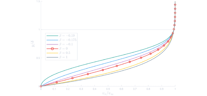
The velocity profiles corresponding to various pressure gradients \(\beta\) are shown in the figure below. A negative pressure gradient, \(\beta > 0\), slightly thins the boundary layer. The viscous deceleration is counteracted by pressure acceleration, resulting in steeper velocity profiles.

A positive pressure gradient, \(\beta < 0\), opposes the flow, slowing down the fluid near the wall even more. The result is a thickened boundary layer and the appearance of an inflection point in the velocity profile. If this effect is strong enough, the flow may reverse and eventually separate. This critical behaviour and its implications for airfoil performance are further discussed in the web post from figure 34.

Velocity profiles over airfoil #

From the different lines for different values of \(\beta\), it is clear that pressure gradients have a strong influence on the shape of the boundary layer velocity profile. Even for a symmetric airfoil at zero incidence, the pressure is not constant along the surface as can be seen in the figure below. As the flow moves from the leading edge to the middle of the airfoil, it accelerates and the pressure decreases. This results in a negative pressure gradient. Beyond the midpoint, the pressure increases again toward the trailing edge, so the flow is decelerated.

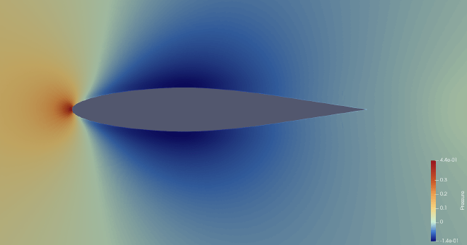
Having identified regions of negative and positive pressure gradients, we now assess whether the corresponding velocity profiles reflect the behaviour expected from flat plate boundary layer theory.

The figure below shows streamwise velocity profiles extracted at three locations along the airfoil surface. The boundary layer thickness \(\delta_{99}\) at each location was computed as the distance from the wall where the tangential velocity equals \(v_x= 0.99v_{\infty}\). Since the flow accelerates along the curved surface of the airfoil, the velocity just outside the boundary layer may exceed the free stream velocity. Strictly, \(\delta_{99}\) should then be based on this local edge velocity, so the values shown somewhat underestimate the boundary layer thickness.

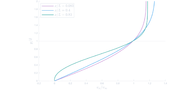
Near the leading edge, the velocity gradient at the wall is steep, characteristic of a thin boundary layer undergoing acceleration due to a negative pressure gradient. In the middle of the airfoil, the profile is most similar to the classic Blasius solution. The pressure gradient here is minimal. Near the trailing edge, however, the profile develops an inflection point, consistent with the presence of a positive pressure gradient. This behaviour agrees with both the flat plate analogy and the description in the original experiment, which says one might anticipate a small separation region near the trailing edge.

Simulation #

To replicate the original figure by H. Werlé in the ONERA water tunnel, the simulation was carried out using Star-CCM+.

Geometry #

The Album of Fluid Motion provides only the airfoil type and the Reynolds number, specified as \(Re_L = 7000\) based on the chord length of the wing. There is more detailed information in the original source [4], which reports that the airfoil has a chord length of \(L = 120\ mm\). Using this and assuming water at \(25\degree C\) is used, the inlet velocity can be determined.

$$ \begin{gather*} Re_L = \frac{\rho v_{\infty} L}{\mu} = 7000 \\ v_{\infty} = \frac{7000 \cdot 8.8871\cdot{10}^{-4}}{997.561 \cdot 0.12} = 0.052\ m/s \end{gather*} $$

The airfoil geometry is generated using TraCfoil, which outputs a dxf file that includes the leading edge radius given in the NACA table [5]. This was then converted to a CSV file that could be opened in Star-CCM+.

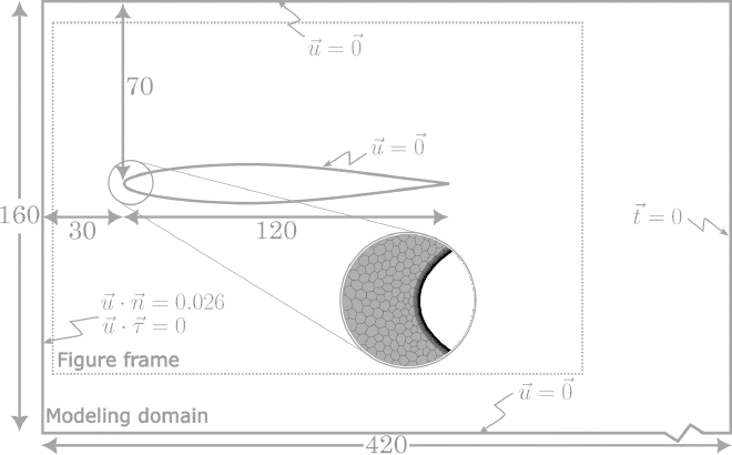
According to [4], the test section of the ONERA water tunnel measures \(10\ mm\) in width and \(160\ mm\) in height. The length is not given, but is assumed to have a negligible effect on the resulting flow field.

Meshing #

Although the flow is described as planar, a 3D polygonal mesh with prism layers was used because it also includes effects of the side walls and it gave more accurate results. A comparison can be found below in the section on inaccuracies. The base size was set to \(0.001\ m\), which gave a total of 4746641 cells. 45 prism layers were used at a height of \(3\cdot 10^{-4} m\).

To reduce computational cost, only half of the water tunnel was modelled. A symmetry boundary condition is applied along the middle of the domain and the other side is assigned a no-slip wall condition. The top and bottom of the domain, as well as the airfoil surface, were also set to no-slip walls.

Physics setup #

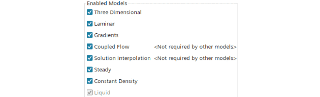
The flow is observed to be laminar, therefore no turbulence model is used. Furthermore, it was assumed to be steady and water was used as the working fluid.

The coupled flow solver is chosen, which requires more computational power, because it solves the velocity and pressure in one system of equations (as opposed to segregated flow, which solves the velocity fields first and then the pressure). Coupled flow is usually used in systems with high speeds, so it seems like it would not make sense to use it in these low-speed systems. However, in practice, the segregated flow solver would not converge, whereas the coupled flow would. In cases where the segregated solver did converge, it was almost always slower to converge than coupled flow, possibly because the coupled flow solver scales linearly with the cell count [6].

The models used can be seen below:

Visualisation #

Paraview was used to visualise the streamlines over the airfoil. This was carried out using the Stream Tracer filter with a point cloud as seed placed at the location of a streamline at the inlet. A Tube filter is then applied to match the colour and thickness seen in the original picture. This was done for each of the 26 streamlines visible in the picture. A CSV file which includes an interpolation of the airfoil geometry was imported and converted to points using the Table To Points filter to visualise the outline of the airfoil. The pipeline can be seen below:

Inaccuracies in results #

The original photograph is described as showing a planar flow, so the simulation was initially carried out using a 2D mesh. But a 3D simulation ended up being more accurate, as shown in the comparison below at the original Reynolds number of \(Re_L = 7000\).

2D

3D

The flow far away from the airfoil is very similar, however, notable differences appear near the surface, particularly near the trailing edge, where the 2D simulation predicts early separation. Although the original description mentioned that one might anticipate a separation region, this is not visible to the same extent as predicted in the 2D result.

To test whether the early separation in 2D is merely a matter of Reynolds number, the 2D simulation was repeated at half the inlet velocity, i.e. at \(Re_L = 3500\).

2D Re = 3500

3D

Causes of differences #

Despite improved results, the 3D simulation does not perfectly reproduce the original flow field. Several factors may contribute:

• The exact placement of the airfoil within the tunnel is not specified. Small differences in position or angle could affect the flow behaviour.
• The CFD model assumes a uniform inflow velocity, but in the water tunnel, there might be slight differences along the inflow boundary.

The combination of these factors could explain the difference between the simulation and the original picture.

References #

[1] Welty J. R., Rorrer G. L., and Foster D. G.. Fundamentals of Momentum, Heat, and Mass Transfer. Wiley, 2019.

[2] Aarseth J. B.. Numeriske beregninger Kompendium. NTNU, 2014.

[3] Hellevik L. R., Numerical methods for engineers. NTNU, 2020. URL: https://leifh.folk.ntnu.no/teaching/tkt4140/._main037.html

[4] Werlé, H.. Le Tunnel hydrodynamique au service de la recherche aérospatiale. O.N.E.R.A 1974

[5] Loftin, L. K., Jr.. Theoretical and experimental data for a number of NACA 6A-Series Airfoil sections. NASA Technical Reports Server (NTRS). 1946. URL: https://ntrs.nasa.gov/citations/20050092351

[6] Siemens Digital Industries Software. Simcenter STAR-CCM+ 2310 User Guide. URL: http://support.sw.siemens.com/en-US/product/226870983