Fig 103. Repetition of Reynolds' dye experiment
Table of Content
“Osborne Reynolds’ celebrated 1883 investigation of stability of flow in a tube was documented by sketches rather than photography. However the original apparatus has survived at the University of Manchester. Using it a century later, N.H. Johannesen and C. Lowe have taken this sequence of photographs. In laminar flow a filament of colored water introduced at a bell-shaped entry extends undisturbed the whole length of the glass tube. Transition is seen in the second of the photographs as the speed is increased; and the last two paragraphs show fully turbulent flow. Modern traffic in the streets of Manchester made the critical Reynolds number lower than the value 13,000 found by Reynolds.”
Large eddy simulation #
Reynolds number and (in)stability #
Reynolds’ 1883 experiment of pipe flow eventually lead to the formulation of the Reynolds number as \( Re = \frac{\rho \hat{U}\hat{L} }{\mu} \), with \( \rho \) and \( \mu \) the fluid’s density and dynamic viscosity, and \( U \) and \( L \) a reference velocity and length. This dimensionless number assigns a value to a flow system so that a similar system operating at a different velocity, with a geometric scaling and/or with different fluid properties will exhibit the same flow phenomena if these values are changed in such a way that the Reynolds number remains the same. This concept forms the foundation for wind tunnel and tow-tank experiments. The mathematical background of the Reynolds number is detailed in Figure 42, where it is indeed shown that, for equal Reynolds number, the non-dimensionalized governing equations are identical.
However, the 1883 experiment primarily identified \( Re \) as an indicator of the stability of the flow. Here, `stability’ should be understood as the tendency of flow to, after some perturbation, either return to a laminar state or develop further into a turbulent state. The images show four instances with increasing Reynolds number from top to bottom. The top image is a stable laminar flow as shown with dye following a straight line. The second image shows the transition from laminar to turbulent flow which was given a value for the Reynolds number of around \(13,000\), the critical Reynolds number. The next two images then show fully turbulent, unstable flows corresponding to a Reynolds number greater than \(13,000\).
For turbulent flows, the Reynolds number has one more interpretation of importance to this study: it dictates the range of scales involved in the flow. Here, “scales” can loosely be interpreted as the differently sized vortical structures (eddies). As the Reynolds number increases, the difference in size between the largest eddies and smallest eddies also increases. The distribution of these eddies in terms of how much kinetic energy is housed in eddies of a certain length follows a particular pattern:
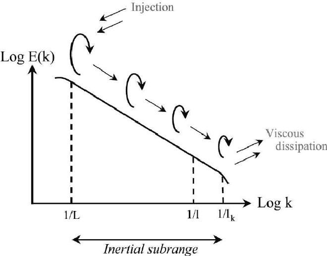
The larger vortices are represented on the left side of the graph and the size of vortices is smaller as you move to the right. As the graph indicates, the larger vortices carry most of the kinetic energy. The vortices interact, and kinetic energy is on average transferred from larger length scales to smaller length scales, where the smallest vortices then dissipate the kinetic energy as heat. This is known as the energy cascade. Kinetic energy can also travel up the stream, which is called “backscatter”. This is how small perturbations to a steady flow can trip turbulence.
Large Eddy Simulation (LES) #
Computationally reproducing this experiment requires careful consideration of the just described physical processes. Clearly, a turbulence model is required. The two available paradigms are (Unsteady) Reynolds-averaged Navier-Stokes ((U)RANS, discussed in Figure 47) and Large Eddy Simulation (LES). (U)RANS involves averaging and thus aims at resolving the left most scales in the above diagram. The corresponding turbulence models are highly dissipative, dampening small perturbations. It will thus not suffice for capturing the sensitive transition phase from laminar to turbulent flow, nor for resolving the flow up to the level of detail required to reproduce the image. For this reason, this study focuses on Large Eddy Simulation.
Large Eddy Simulation (LES) provides the means to simulate a range of the scales that form in the turbulent fluid flow. It is just below direct numerical simulation (DNS) in terms of computational expense, and the key difference between the two is the use of a filter to remove the vortices that are too small to resolve on the computational mesh. The effect of these eliminated small vortices must be incorporated in the model for the large vortices in the form of a subgrid-scale model. This process greatly decreases the computational expense in comparison to DNS, which resolves the full range of scales.
The quality and level of detail provided by LES is highly dependent on the mesh size as this dictates the permissible filter width. The finer the mesh, the more eddies can be resolved and the less must be modeled with the subgrid-scale models. It is generally accepted that an LES simulation should solve around 80% of the turbulent kinetic energy of the flow, leaving 20% to be represented by the subgrid-scale model. As a consequence, LES models require refinement with increasing Reynolds number, as we’ve seen that this widenes the complete scale range. Techniques for estimating the required mesh-size to capture 80% of the kinetic energy exist and are the topic of a later post.
Filtered Navier-Stokes equations #
LES is based on a modified version of the Navier-Stokes equations, which are the equations that describe mass and momentum (and sometimes energy) balance. In the incompressible case, they read:
$$ \begin{cases} \rho \frac{\partial \boldsymbol{u}}{\partial t} +\nabla \cdot ( \rho \boldsymbol{u} \oplus \boldsymbol{u} ) = \mu \nabla^2 \boldsymbol{u} - \nabla p \\ \nabla\cdot \boldsymbol{u} = 0 \end{cases} $$
If these equations were to be solved exactly (e.g., by DNS), one obtains the velocity and pressure fields in full detail (i.e., with their full range of scales).
To compute only the larger scales, one needs a way to formally separate them from the small scales. In LES, this is performed with a filter:
$$ \mathcal{F} \boldsymbol{u}(\boldsymbol{x},t) = \bar{\boldsymbol{u}}(\boldsymbol{x},t) $$
where \( \mathcal{F} \) is the filtering operator and \( \bar{\boldsymbol{u}} \) the filtered solution. Many types of filters exist, each with their own properties, but in general you can think of them as the blurring operation known from image editing. The evolution equations governing the filtered velocity and pressure field \( ( \boldsymbol{\bar{u}}(x,t), \bar{p}(x,t) ) \) are then obtained by filtering the Navier-Stokes equations [1]:
$$ \begin{cases} \rho \frac{\partial \bar{\boldsymbol{u}} }{\partial t} +(\nabla \cdot \rho \bar{\boldsymbol{u}} \oplus \bar{\boldsymbol{u}} ) = \mu \nabla^2 \bar{\boldsymbol{u}} - \nabla \bar{p} -\nabla\cdot\boldsymbol{\tau} \\ \nabla\cdot \bar{\boldsymbol{u}} = 0 \end{cases} $$
The crucial part of these equations is the occurence of the tensor \(\tau_{ij} = \rho (\overline{u_iu_j} - \bar{u}_i \bar{u}_j)\), called the subgrid-scale stress. Mind you, it is not really a stress (rather, it is the difference between the convective transport of the filtered solution and the filtered convective transport of the solution), but in the way that the tensor manifests itself in the equations it is indistinguishable from a stress. Once an expression for this tensor is substituted in terms of the filtered quantities, the filtered equations can be solved for the pair \( ( \boldsymbol{\bar{u}}(x,t), \bar{p}(x,t) ) \). The chosen expression for \( \boldsymbol{\tau} \) is called the subgrid-scale model.
Subgrid-scale models #
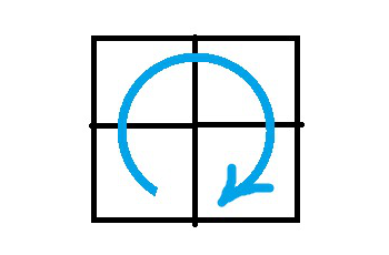
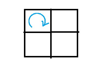
The particular form of the subgrid-scale (SGS) model inevitably relates to the filter width \( \Delta \), and hence effectively to the cell size of the mesh. Conceptually, it takes at least 4 cells to capture an eddie as illustrated in the below images. As such, SGS models should only model eddies of length scales smaller than the individual cells.
Most LES subgrid-scale stress models are based on the eddy-viscosity assumption. Proposed by Boussinesq in 1877, it hypothesizes that the dissipative nature of the smallest eddies in the flow effectively increases the viscosity of the fluid. This naturally leads to:
$$ \tau_{ij} = \frac{2}{3} k \delta_{ij} - 2 \mu_{SGS} \bar{S} _{ij} $$
where \(k\) is the turbulent kinetic energy, \(\mu_{SGS}\) is the SGS eddy-viscosity and \(k\) is the filtered strain-rate tensor \( \bar{S} _{ij} = \frac{1}{2} (\frac{\partial \bar{u}_i}{\partial x_j} + \frac{\partial \bar{u}_j}{\partial x_i}) \).
Also within the class of eddy-viscosity models there exist many variations. The models that we focus on are the Smagorinsky model and the Wall-Adapting Local Eddy-viscosity (WALE) model.
Smagorinsky:
$$ \mu_{SGS} = (C_S \Delta)^2 \sqrt{ 2 \bar{S} _{ij} \bar{S} _{ij} } $$
WALE:
$$ \mu_{SGS} = (C_W \Delta)^2 \sqrt{ f(\bar{\boldsymbol{S}}) } $$ Refer to [2] for the exact definition of \( f(\bar{\boldsymbol{S}}) \).
The Smagorinsky model is the base model from which all other models are adapted. The WALE model is a particular version that exhibits almost zero eddy-viscosity when the flow is laminar. This feature makes it well suited for modeling the laminar to turbulent transition, the focus of this work. Additionally, it provides a more accurate decay of eddy-viscosity at near wall regions, hence being wall-adapting [2]. Pipe flow is highly wall bounded, making this an important factor.
Simulation #
Perturbation of equilibrium state #
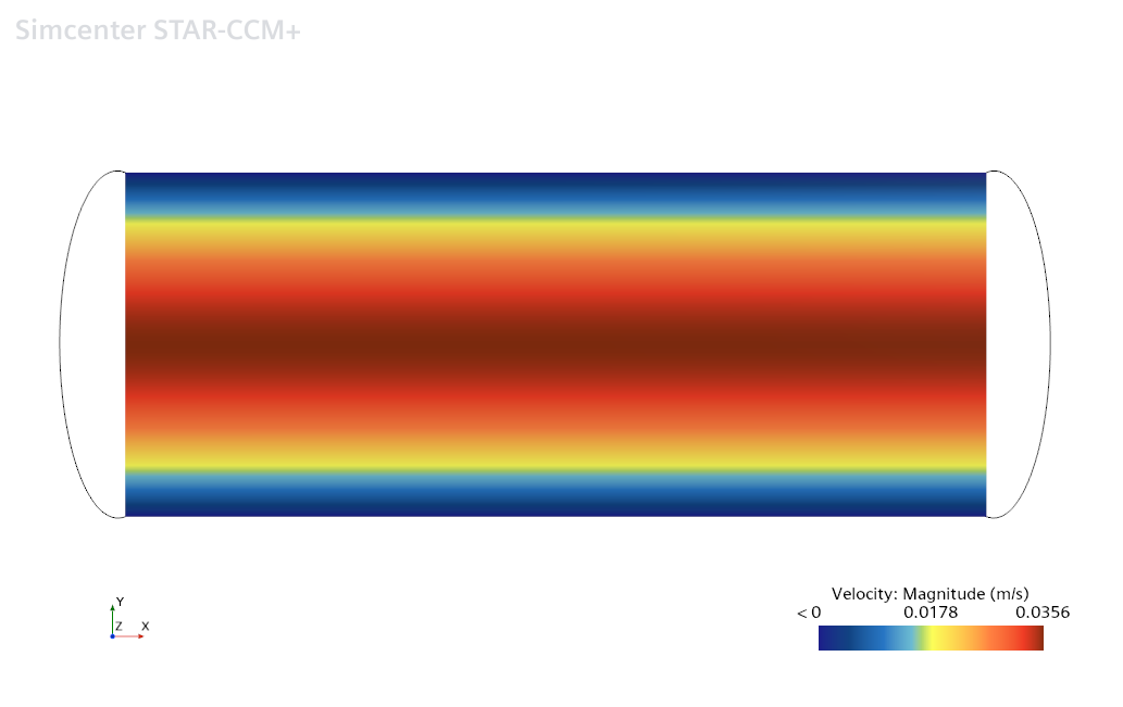
To reproduce the Reynolds dye experiment, we perturb the equilibrium state at an increasingly higher Reynolds number. Past the critical Reynolds number, the perturbation does not damp out (= steady equilibrium), but rather grows and leads to turbulent flow (= unsteady equilibrium). The equilibrium velocity profile of pipe flow does not depend on the Reynolds number: it is the parabolic Poiseuille flow profile:
$$ U(r) = \frac{1}{4 \mu} \frac{dP}{dx}(r^2-R^2) $$ where \(\mu\) is the dynamic viscosity, \( \frac{dP}{dx} \) is the mean pressure gradient, and \(R\) the pipe radius.
In the experiment, the fluid is driven through the pipe by a pressure gradient. This pressure gradient can be modelled as a momentum source, a vector quantity that gives the magnitude and direction of the body force acting on the fluid. With the above expression for the Poiseuille flow, the required body force to hit a target Reynolds number can be derived as:
$$ \boldsymbol{f} = \frac{dP}{dx} \boldsymbol{e}_x = Re \frac{2\mu^2}{\rho R^3} \boldsymbol{e}_x $$
where it must be noted that the Reynolds number is then based on the center velocity of the laminar Poiseuille flow, which is anticipated to be a severe overprediction compared to the (unspecified) reference velocity taken in the experimental photographs.
The perturbation to this equilibrium state is introduced in the form of a synthetic eddy method. As parameters, this takes values for the turbulence intensity and turbulent length scale, for which we use the following expressions:
$$ I = 0.7 \sqrt{\frac{\frac{3}{2} v_t^2}{U^2}} $$
$$ L_s = 0.07 D $$
where \(v_t\) is the turbulent velocity scale which is 10% of the free stream velocity (\(U\)). The intensity is multiplied by a factor \(0.7\) to reduce the intensity of the perturbation and uncover the intrinsic stability characteristics of the flow.
The simulations are then run for 90 seconds of real time to allow the flow to reach a statistically steady state where it is no longer affected by the initial perturbation. Instead, it either returns to the laminar state or remains in a turbulent state depending on the system’s stability.
Computational set-up #
To model this system, we define the pipe domain as having a diameter of \(100 mm\) and a length of \(500 mm\). The open ends of the pipe are connected with periodicity conditions. In this way, there is no real inlet and outlet, but instead the flow moving through the outlet is reintroduced at the inlet. It can be interpreted as stacking many small pipe segments next to one another to create an infinitely long pipe. This ensures that the flow can fully develop, and the progression of turbulence is not limited by the pipe length.
This domain is then meshed with a trimmed cell mesher. The geometry is divided into equally sized cubes of \(2 mm\), which are trimmed and subdivided to fit the domain boundary and provide a moderately well refined boundary layer mesh. This leads to a total of 400,000 grid cells.
On top of the mesh resolution, the quality of LES also depends on the temporal resolution. The accuracy of the results are dependent on time-step size, as characterized by the so-called Courant number. The Courant number is a dimensionless number indicating how many cells of distance a fluid particle travels per time-step. It is defined as:
$$ C = |\boldsymbol{u}| \frac{\Delta t}{\Delta x} $$
where \(\boldsymbol{u}\) is the fluid velocity, \(\Delta t\) is the timestep size, and \(\Delta x\) is the mesh cell size.
For LES, good practice is to keep the Courant number below one. Then, during each time-step, the flow will at most move one cell length across. This ensures that there is sufficient amount ‘communication time’ between the cells in the mesh; if the Courant number exceeds a value of one the fluid would be “skipping over” cells. For this study, we use a Courant number of \(0.9\).
Visualization #
The flow is visualized in
Paraview. Since a limited length of the pipe is simulated, the first step is to extend the pipe during post-processing. This is done by opening multiple of the exported Ensight Gold file and then using the transform filter to translate these datasets to be next to one another to form a longer pipe. The data must be shared across these datasets, so the group datasets, merge blocks, and append datasets filters are used. This essentially makes the datasets uniform so that, as the flow passes through the periodic boundary, it is displayed on the next dataset in line.
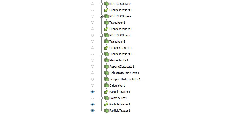
The next step is to visualize a stream of dye moving through the flow. Since data is exported as cell data when simulating, the cell to point data filter is utilized. The point data can then be used to calculate the velocity vectors of the flow within the calculator. To simulate the dye, the particle tracer filter is given a point source from which the dye flow is initiated, and propagated by the velocity values found with the calculator. The Paraview pipeline is shown below:
With this visualization, we are able to get results which are a qualitative match with the images in the experiment. Though the turbulent cases are naturally not identical to the experiment due to the unpredictability of turbulence, the characteristics are similar. The key similarities are in the frequency and amplitude of the vortices, and the thinning of the dye.
The main discrepancy is that our LES simulation of the transitioning flow exhibits stronger turbulent features than the flow in the photograph. This is most likely due to our conservative estimate of the Reynolds number, as described before. The actual Reynolds number of the LES simulation would have to be determined a-posteriori and iterated upon.
References #
[1] Stephen B Pope. Turbulent Flows. Cambridge University Press (2020).
[2] Minwoo Kim et al. “Assessment of the wall-adapting local eddy-viscosity model in transitional boundary layer”. In: Computer Methods in Applied Mechanics and Engineering 371 (2020), p. 113287. doi: 10.1016/J.CMA.2020.113287.