Fig 47. Circular cylinder at R=2000

Experiment

Simulation

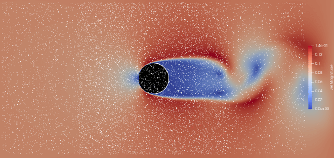
“Air bubbles in water show the velocity field of a flow around a circular cylinder at Reynolds number \(Re = 2000\). At this Reynolds number, there is a clear boundary layer separation followed by an oscillating turbulent wake. For comparison, a transient simulation was created in Simcenter StarCCM+ using the SST turbulence model.” Photograph by ONERA photograph, Werlé & Gallon 1972

Theory #

Turbulent flow #

Turbulent flow is characterized by its chaotic and irregular behaviour. Although turbulent flow is often encountered and widely relevant to engineers, accurately modelling and predicting it has been the subject of intense scientific research over the past few decades. In contrast to the predictable and easy to model laminar flow, turbulent flow requires complex models to solve the million dollar Navier-Stokes equations. $$ \rho (\frac{\partial\textbf{u}}{\partial t} + \textbf{u}\cdot \nabla \textbf{u}) = -\nabla p + \nabla \cdot (\mu (\nabla \textbf{u} + (\nabla \textbf{u}^T))-\frac{2}{3}\mu(\nabla \cdot \textbf{u})\textbf{I}) + \textbf{F} $$ Numerically solving the Navier-Stokes equations is extremely computationally expensive because of the largely different mixing-length scales present in turbulent flow. From modelling planet sized meteorological effects such as rotating tropical cyclones to modelling microscopic effects of vortex energy dissipation due to viscous losses, the Navier-Stokes equations need to be adjusted for numerical computations.

Reynolds-averaged-Navier-Stokes #

The Reynolds-averaged Navier-Stokes equations (RANS) choose to model turbulence effects on the mean flow scale. This is done with the so-called Reynolds decomposition, which decomposes a quantity \(u(x,y,z,t)\) into its mean and fluctuating part. $$ u(x,y,z,t) = \overline{u(x,y,z)} + u’(x,y,z,t) $$ Deriving the RANS equations for stationary, incompressible fluid flow starts with the standard Navier-Stokes equations for stationary incompressible fluid flow. Using the Einstein summation convention and substituting the dynamic viscosity \(\mu\) with the kinematic viscosity \(\nu = \mu / \rho\), these Navier-Stokes equations can be written as $$ \frac{\partial u_i}{\partial t} + u_j \frac{\partial u_i}{\partial x_j} = -\frac{1}{\rho} \frac{\partial p}{\partial x_i} + \nu \frac{\partial ^2 u_i}{\partial x_j \partial x_j} $$ Applying the Reynolds decomposition to the quantities \(u\) and \(p\) and time-averaging the resulting equation, one is left with the following equation. $$ \frac{\partial \overline{u}_i}{\partial t} + \overline{u}_j \frac{\partial \overline{u}_i}{x_j} + \overline{u_j’ \frac{\partial u_i’}{\partial x_j}} = -\frac{1}{\rho} \frac{\partial \overline{p}}{\partial x_i} + \nu \frac{\partial^2 \overline{u}_i}{\partial x_j \partial x_j} $$ \(\overline{u_j’ \frac{\partial u_i’}{\partial x_j}}\) is the only term that cannot be directly time-averaged. However, by applying the chain rule and the law of conservation of mass, it can be shown that $$ \overline{\frac{\partial u_i’}{\partial x_j} u_j’} = \frac{\partial}{\partial x_j} \overline{u_i’ u_j’} $$

The detailed derivation can be found here.

Applying the chain rule to \(\frac{\partial}{\partial x_j} \overline{u_i’ u_j’}\) leads to $$ \frac{\partial}{\partial x_j} \overline{u_i’ u_j’} = \overline{\frac{\partial u_i’}{\partial x_j} u_j’} + \overline{\frac{\partial u_j’}{\partial x_j} u_i’} $$ Yet the law of conservation of mass says that \(\frac{\partial u_j}{\partial x_j} = 0\) and thus the term above can be simplified to $$ \frac{\partial}{\partial x_j} \overline{u_i’ u_j’} = \overline{\frac{\partial u_i’}{\partial x_j} u_j’} $$

Multiplying \(\overline{u_i’ u_j’}\) by \(\rho\) is known as the Reynolds stress term and can be substituted in the Reynolds-averaged equation above. Rearranging and factoring the right-hand side of the aforementioned equation results in the so-called Reynolds-averaged Navier–Stokes (RANS) equation. $$ \overline{u}_j \frac{\partial \overline{u}_i}{x_j} = -\frac{1}{\rho} \frac{\partial \overline{p}}{\partial x_i} + \frac{\partial}{\partial x_j} \left(\mu \frac{\partial \overline{u}_i}{\partial x_j} - \rho \overline{u_i’ u_j’} \right) $$ The RANS equations are the basis for all RANS turbulence models including the shear stress transport (SST), k-omega and k-epsilon models. More specifically, these models are based on the Reynolds stresses \(\rho \overline{u_i’ u_j’}\) from the above RANS equation.

In 1945, P.Y. Chou gave a very complicated closure equation for the time evolution of the Reynolds stress [1]. Tracing \(\overline{u_i’u_j’}\) in the said equation would lead to the turbulent kinetic energy \(k\) and \(\nu \overline{\frac{\partial u_i’}{\partial x_k} \frac{\partial u_j’}{\partial x_k}}\) is known as the turbulent dissipation rate \(\epsilon\). Most RANS models are based on the above mentioned equation or on the simpler Boussinesq eddy viscosity hypothesis expressed below [2]. $$ \rho \overline{u_i’ u_j’} = \frac{2}{3} \rho k \delta_{ij} - \mu_t \left( \frac{\partial \overline{u_i}}{\partial x_j} + \frac{\partial \overline{u_j}}{\partial x_i} \right) $$

k-epsilon turbulence model #

As the name suggests, the k-epsilon turbulence model is based on the turbulent kinetic energy \(k\) and the turbulent dissipation rate \(\epsilon\). These two quantities are based on the two ends of the eddy size spectrum. \(k\) being the turbulent kinetic energy conserved in large, energy dense vortices and \(\epsilon\) being the conversion rate from kinetic energy to thermal energy through viscous forces in microscopic eddies. The original model developed by Jones and Launder [3] prescribes the following transport equations for \(k\) and \(\epsilon\):

$$ \begin{align*} \frac{\partial \rho k}{\partial t} + \frac{\partial \rho k u_i}{\partial x_i} &= \frac{\partial}{\partial x_j} \left( \frac{\mu_t}{\sigma_k} \frac{\partial k}{\partial x_j} \right) + P_k - \rho \epsilon \\ \frac{\partial \rho \epsilon}{\partial t} + \frac{\partial \rho \epsilon u_i}{\partial x_i} &= \frac{\partial}{\partial x_j} \left( \frac{\mu_t}{\sigma_{\epsilon}} \frac{\partial \epsilon}{\partial x_j} \right) + C_{1\epsilon} \frac{\epsilon}{k} P_k - C_{2\epsilon} \frac{\rho \epsilon^2}{k} \end{align*} $$

with the eddy viscosity \(\mu_t\) modelled as $$ \mu_t = \rho C_{\mu} \frac{k^2}{\epsilon} $$ and the production of \(k\) modelled as $$ P_k = - \rho \overline{u_i’u_j’} \frac{\partial u_j}{\partial x_i} $$ Being able to model the eddy viscosity \(\mu_t\) with \(k\) and \(\epsilon\), provides a closure equation to the RANS equations, since \(\mu_t\) is needed in the Boussinesq eddy viscosity hypothesis for the Reynolds stresses. Thus, the RANS equations can be solved.

As is well known from literature [4], the main drawback of the k-epsilon model is its poor prediction of energy dissipation in viscous sublayers and adverse pressure gradients. More specifically, the k-epsilon model struggles to determine energy dissipation in scenarios where viscous forces are dominant. A potential solution to this is the so-called low Reynolds number k-epsilon model (low-Re k-epsilon), which uses damping functions on the empirical coefficients \(C_{1 \epsilon}\), \(C_{2 \epsilon}\) and \(C_{\mu}\) in near wall regions. However, these empirical damping functions are based on a simple experiment with flow over a spinning disc [5], which inherently makes this model less accurate in other situations. Unfortunately, most engineering industries encounter many different types of turbulent flows, which is where the need for a better suited model arises.

k-omega turbulence model #

The motivation behind the development of recent k-omega models is to make up for what even the low-Re k-epsilon model lacks in near-wall and adverse pressure gradient prediction accuracy. Although the k-omega and k-epsilon models are very similar and based on the same assumptions for the RANS equations, the key difference is the need for empirical damping functions on the coefficients of the low-Re k-epsilon model and the absence of these for the k-omega model.

The k-omega and k-epsilon model are closely related through the following expression. $$ \omega = \frac{\epsilon}{C_{\mu}k} \quad \quad C_{\mu} = 0.09 $$ While the transport equation for \(k\) remains practically the same for both models, plugging the above expression into the transport equation for \(\epsilon\) yields the k-omega model. $$ \begin{align*} \frac{\partial k}{\partial t} + \frac{\partial k u_i}{\partial x_i} &= \frac{1}{\rho} \frac{\partial}{\partial x_j} \left[ \left( \mu + \frac{\mu_t}{\sigma_k} \right) \frac{\partial k}{\partial x_j} \right] + P_k - \beta^* \omega k \\ \frac{\partial \omega}{\partial t} + \frac{\partial \omega u_i}{\partial x_i} &= \frac{1}{\rho} \frac{\partial}{\partial x_j} \left[ \left( \mu + \frac{\mu_t}{\sigma_{\omega}} \right) \frac{\partial \omega}{\partial x_j} \right] + \frac{\gamma \omega}{k} P_k - \beta \omega^2 \end{align*} $$ Although new empirical coefficients need to be computed for this model, there is no need for empirically developed damping functions for the coefficients, which makes this model more generally applicable.

k-omega SST turbulence model #

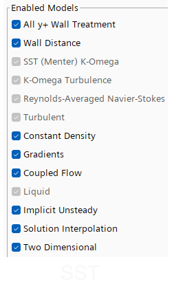
The simulation that provided the data for the comparison figure at the top of the page was run using Menter’s SST turbulence model [6]. Also known as the k-omega SST model, this turbulence model combines the strengths of both the k-epsilon and k-omega model by making use of both models at the same time. Using a blending function the k-epsilon model is activated in the freestream areas of the domain and the k-omega model is activated in near-wall and adverse pressure gradient regions.

To start things off, the k-omega model can be left in it’s original form as developed by Wilcox, but the k-epsilon model needs to be expressed in terms of \(\omega\) using \(\epsilon = \omega k\). Using the Lagrangian derivative on the left-hand side and expressing the production term \(P_k\) with the Reynolds stress \(P_k = \tau_{ij} \frac{\partial u_i}{\partial x_j}\), the transport equation of \(\epsilon\) in terms of \(\omega\) is expressed below. $$ \rho \frac{D k}{D t} = \frac{\partial}{\partial x_j} \left( \frac{\mu_t}{\sigma_k} \frac{\partial k}{\partial x_j} \right) + \tau_{ij}\frac{\partial u_i}{\partial x_j} - \rho \omega k $$

The full derivation including a double chain rule expansion and the substitution of the transport equation for \(k\) can be found here.

The next step in the transformed k-epsilon model derivation is to express the original transport equation for \(\epsilon\) in terms of \(\omega\). Applying the chain rule on the left-hand side and in the diffusion term leads to $$ \rho \frac{D \omega}{D t} k + \rho \frac{D k}{D t} \omega = \frac{\partial}{\partial x_j}\left( \frac{\mu_t}{\sigma_{\epsilon}} \frac{\partial \omega}{\partial x_j} k \right) + \frac{\partial}{\partial x_j}\left( \frac{\mu_t}{\sigma_{\epsilon}} \frac{\partial k}{\partial x_j} \omega \right) + C_1 \omega \tau_{ij}\frac{\partial u_i}{\partial x_j} - C_2 \rho \omega^2 k $$ The chain rule still needs to be applied to the following terms. $$ \begin{split} \frac{\partial}{\partial x_j}\left( \frac{\mu_t}{\sigma_{\epsilon}} \frac{\partial \omega}{\partial x_j} k \right) + \frac{\partial}{\partial x_j}\left( \frac{\mu_t}{\sigma_{\epsilon}} \frac{\partial k}{\partial x_j} \omega \right) &= \frac{\partial}{\partial x_j}\left( \frac{\mu_t}{\sigma_{\epsilon}} \frac{\partial \omega}{\partial x_j} \right) k + \frac{\mu_t}{\sigma_{\epsilon}}\left( \frac{\partial k}{\partial x_j} \frac{\partial \omega}{\partial x_j} \right) \\ &+\frac{\partial}{\partial x_j}\left( \frac{\mu_t}{\sigma_{\epsilon}} \frac{\partial k}{\partial x_j} \right) \omega + \frac{\mu_t}{\sigma_{\epsilon}}\left( \frac{\partial k}{\partial x_j} \frac{\partial \omega}{\partial x_j} \right) \end{split} $$ Regrouping these terms before plugging them into the equation above and isolating \(\frac{D \omega}{D t}\) leads to $$ \begin{split} \rho \frac{D \omega}{D t} &= \frac{\partial}{\partial x_j}\left( \frac{\mu_t}{\sigma_{\epsilon}} \frac{\partial \omega}{\partial x_j} \right) + \frac{2}{k} \frac{\mu_t}{\sigma_{\epsilon}}\left( \frac{\partial k}{\partial x_j} \frac{\partial \omega}{\partial x_j} \right) + \frac{\omega}{k} \frac{\partial}{\partial x_j}\left( \frac{\mu_t}{\sigma_{\epsilon}} \frac{\partial k}{\partial x_j} \right) + C_1 \frac{\omega}{k} \tau_{ij}\frac{\partial u_i}{\partial x_j} \\ &- C_2 \rho \omega^2 - \rho \frac{D k}{D t} \frac{\omega}{k} \end{split} $$ The transformed transport equation for \(k\) can now be substituted into the equation above. $$ \begin{split} \rho \frac{D \omega}{D t} &= \frac{\partial}{\partial x_j}\left( \frac{\mu_t}{\sigma_{\epsilon}} \frac{\partial \omega}{\partial x_j} \right) + \frac{2}{k} \frac{\mu_t}{\sigma_{\epsilon}}\left( \frac{\partial k}{\partial x_j} \frac{\partial \omega}{\partial x_j} \right) + \frac{\omega}{k} \frac{\partial}{\partial x_j}\left( \frac{\mu_t}{\sigma_{\epsilon}} \frac{\partial k}{\partial x_j} \right) + C_1 \frac{\omega}{k} \tau_{ij}\frac{\partial u_i}{\partial x_j} - C_2 \rho \omega^2 \\ &- \frac{\omega}{k} \frac{\partial}{\partial x_j}\left( \frac{\mu_t}{\sigma_k} \frac{\partial k}{\partial x_j} \right) - \frac{\omega}{k} \tau_{ij}\frac{\partial u_i}{\partial x_j} + \rho \omega^2 \end{split} $$ Regrouping these terms leads to a very similar equation that can be found in this paper [7, eq (26)]. $$ \begin{split} \rho \frac{D \omega}{D t} &= \frac{\partial}{\partial x_j}\left( \frac{\mu_t}{\sigma_{\epsilon}}\frac{\partial \omega}{\partial x_j} \right) + \frac{\omega}{k} \frac{\partial}{\partial x_j} \left[ \left( \frac{1}{\sigma_{\epsilon}} - \frac{1}{\sigma_k} \right) \mu_t \frac{\partial k}{\partial x_j} \right] + (C_1 -1) \frac{\omega}{k} \tau_{ij} \frac{\partial u_i}{\partial x_j} - (C_2 -1) \rho \omega^2 \\ &+ \frac{2}{k} \frac{\mu_t}{\sigma_{\epsilon}} \left( \frac{\partial k}{\partial x_j} \frac{\partial \omega}{\partial x_j} \right) \end{split} $$ However, for simplification purposes, it can be assumed that \(\sigma_{\epsilon} = \sigma_k\). On top of this, it is known that $$ \mu_t = \rho \frac{k}{\omega} \quad \quad \nu_t = \frac{k}{\omega} $$ Thus, \(\frac{\omega}{k}\) can be replaced with \(\frac{1}{\nu_t}\) and \(\frac{\mu_t}{k}\) can be replaced with \(\frac{\rho}{\omega}\). The following equation is very similar to the one found in Pope’s book “Turbulent Flows” [8, eq (10.94)]. $$ \rho \frac{D \omega}{D t} = \frac{\partial}{\partial x_j}\left( \frac{\mu_t}{\sigma_{\epsilon}} \frac{\partial \omega}{\partial x_j} \right) + (C_1 -1) \frac{1}{\nu_t} \tau_{ij}\frac{\partial u_i}{\partial x_j} - (C_2 -1) \rho \omega^2 + \rho \frac{2}{\omega \sigma_{\epsilon}} \frac{\partial k}{\partial x_j} \frac{\partial \omega}{\partial x_j} $$

The final form of the transformed k-epsilon model as can be found in Menter’s original paper is expressed below. $$ \rho \frac{D \omega}{D t} = \frac{\partial}{\partial x_j} \left[ \left( \mu + \sigma_{\omega 2} \mu_t \right) \frac{\partial \omega}{\partial x_j} \right] + \gamma_2 P_{\omega} - \rho \beta_2 \omega^2 + 2 \rho \sigma_{\omega} \frac{1}{\omega} \frac{\partial k}{\partial x_j} \frac{\partial \omega}{\partial x_j} $$ This equation closely resembles the transport equation of \(\omega\) in the k-omega model, except for the additional cross-diffusion term. Finally, the standard k-omega model can be multiplied with the blending function \(F_1\) and the transformed k-epsilon model can be multiplied with the blending function \((1-F_1)\). The corresponding equations can be added together to give what is known as the baseline model (BSL). $$ \begin{split} \rho \frac{D k}{D t} &= \frac{\partial}{\partial x_j} \left[ \left( \mu + \sigma_k \mu_t \right) \frac{\partial k}{\partial x_j} \right] + \tau_{ij}\frac{\partial u_i}{\partial x_j} - \rho \omega k \\ \rho \frac{D \omega}{D t} &= \frac{\partial}{\partial x_j} \left[ \left( \mu + \sigma_{\omega} \mu_t \right) \frac{\partial \omega}{\partial x_j} \right] + \frac{\gamma}{\nu_t} P_{\omega} - \beta \rho \omega^2 + 2 \rho (1 - F_1) \sigma_{\omega 2} \frac{1}{\omega} \frac{\partial k}{\partial x_j} \frac{\partial \omega}{\partial x_j} \end{split} $$ Since this model is a blend of two models, so are the constants. If \(\phi_1\) represents the constants of the original k-omega model and \(\phi_2\) represents the constants of the transformed k-epsilon model, then the constants \(\phi\) of the BSL model are represented by $$ \phi = F_1 \phi_1 + (1-F_1) \phi_2 $$ All of the constants and exact definition of the blending function \(F_1\) are given in the appendix of the original paper by Menter. What is important to know is that the blending function\(F_1\) is designed such that it is equal to one in the near-wall region and zero away from the surface.

According to Menter, the BSL model behaves very similarly to the standard k-omega model, without the freestream turbulence dependence, which is a considerable improvement. However, the seemingly small difference between the BSL model and the shear stress transport model is what makes the SST model far superior in predicting adverse pressure gradient boundary layer flows. The difference between these two models lies in the definition of the eddy viscosity \(\nu_t\). Namely, the BSL model does not account for the transport of the principal turbulent shear stress, otherwise known as the Reynolds stress. In the SST model, the eddy viscosity is modelled as $$ \nu_t = \frac{a_1 k}{\max(a_1 \omega ; \Omega F_2)} $$ with \(\Omega = \frac{\partial u_i}{\partial x_j}\) and \(F_2\) being one for boundary-layer flows and zero for freestream flows. This simply guarantees that \(\nu_t = \frac{k}{\omega}\) in boundary-layer flows and that the Reynolds-stresses are not over predicted in freesteam conditions.

Turbulence model comparisons #

Directly comparing the k-omega and low-Re k-epsilon models in the same transient simulation environment reveals that they lead to very different solution fields. The k-omega model clearly shows a (potentially over-exagerated) oscillating turbulent wake with many differently sized eddies forming right behind the cylinder, whereas the low-Re k-epsilon model struggles to reach any kind of turbulent oscillation and seems to be depicting stable recirculating eddies, even after a considerable number of calculation iterations. It is important to note that in this particular simulation, the residuals of the standard k-epsilon model did not converge, which is why the low-Re k-epsilon model was used. Comparing the k-epsilon and k-omega models to the SST model used for the visualization at the top of the page, it becomes clear that the SST model is able to provide the closest replication to the experiment.

k-omega

low-Re k-epsilon

To further highlight the difference between all of the turbulence models used, the lift coefficient of the cylinder was plotted while running the simulations. These plots are shown below.

A more in-depth comparison and analysis between the different turbulence models using a different experiment and simulations setups can be found in this post and in this post about flow over a \(2.5^{\circ}\) inclined plate at \(Re = 10000\) and \(Re = 50000\) respectively. More results can also be found on this page about flow over a larger angle inclined plate.

Simulation #

All of the above simulations were carried out in Simcenter StarCCM+. RANS equations and turbulence models based on them can be derived and are valid for 2D cases. This allowed the simulations to be run in 2D and save on computational expenses.

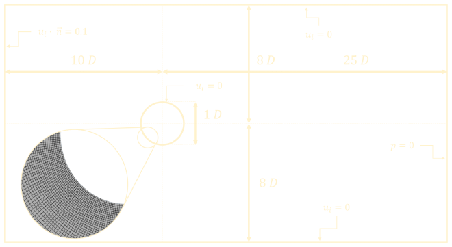
Computational domain #

The computational domain, boundary conditions and finite volume mesh were created based on the information available in the caption of the original figure. It is know that the Reynolds number \(Re=2000\) and that the experiment is set up with water flowing around a circular cylinder. From \(Re = \frac{\rho u D}{\mu}\) the cylinder diameter and inlet velocity can be calculated to be \(D = 0.2\ m\) and \(u = 0.1\ m/s\). The computational domain can be seen in the figure below. The top and bottom walls are located \(8D\) away from the center of the cylinder, as is mentioned in the caption of Figure 44 from the book, which has the same experimental setup as this figure. In the computational domain, the walls and the cylinder have a no-slip boundary condition applied to them, while the inlet is specified as a velocity inlet and the outlet a pressure outlet.

StarCCM+ has quite extensive meshing options and allows for very precise control over the finite volume mesh. The mesh created for this simulation is a quadrilateral mesh with a base size of \(0.2\ m\). However, this base size is only applied to the outermost parts of the domain, as there is a large area around the cylinder and \(6D\) behind the cylinder where mesh refinement with a base size of \(2.5 \cdot 10^{-4}\ m\) and growth rate of \(1.1\) is applied. The total cell count is 25576. Some visual representations can be seen below.

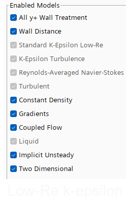
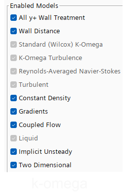
StarCCM+ setup #

The simulation was run as a transient simulation for a total of three times; once using Menter’s SST turbulence model, once using the low Reynolds number k-epsilon turbulence model and a final time using Wilcox’s (2008) k-omega turbulence model. The turbulence model parameters were left in their default configuration and the exact simulation parameters are shown in the figures below. For each of these, a second order implicit unsteady solver with a time-step of \(0.025\ s\) was used. The stopping criteria was set to 50 maximum inner iterations and \(20\ s\) maximum physical time. This means a total of 800 timesteps and 40.000 iterations. The velocity and pressure data was exported to Ensight Gold case files for further post processing.

Visualization #

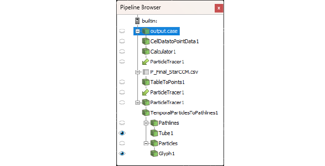
Post processing and visualization is done in Paraview. The ParaView pipeline is shown in the figures below. After importing the simulation data, it first needs to be processed a bit. Namely a CellDataToPointData filter as well as the Calculator filter need to be applied in order to compute the velocity vector from the x-velocity and y-velocity data. Next, in order to achieve a similar visualization as the original figure, particles need to be injected into the velocity field. For this, a point coordinate matrix is created in MATLAB:

k = 0.6;                                % parameter for increasing point concentration      
    
%% General point cloud

P1 = zeros((k*12000)+1,3);              % allocating matrix (3D)
P1(1,:) = [1,2,3];                      % First row description for ParaView

X1 = randi([-1000,1000],k*12000,1);     % 7200 random x-coordinates between 300 and 1200
X1 = X1/10000;                          % dividing by 1e04 to scale coordinates
Y1 = randi([-500,500],k*12000,1);       % 7200 random x-coordinates between 800 and 1200
Y1 = Y1/10000;                          % dividing by 1e04 to scale coordinates
P1(2:end,1) = X1;                       % adding x-coordinates to P matrix
P1(2:end,2) = Y1;                       % adding y-coordinated to P matrix

%% Fine point cloud behind cylinder

P2 = zeros((k*10000)+1,3);              % allocating matrix (3D)
P2(1,:) = [1,2,3];                      % First row description for ParaView

X2 = randi([-500,500],k*10000,1);       % 6000 random x-coordinates between 300 and 1200
X2 = X2/10000;                          % dividing by 1e04 to scale coordinates
Y2 = randi([-500,500],k*10000,1);       % 6000 random x-coordinates between 800 and 1200
Y2 = Y2/10000;                          % dividing by 1e04 to scale coordinates
P2(2:end,1) = X2;                       % adding x-coordinates to P matrix
P2(2:end,2) = Y2;                       % adding y-coordinated to P matrix

%% Points around cylinder (back half)
n = 180;                                % number of points

angles = linspace(0.5*pi, 1.5*pi, n);   % points equally distributed
radius = 0.0101;                        % radius of cylinder + margin
xCenter = 0;                            % Coordinates of center point
yCenter = 0;
X3 = -radius * cos(angles) + xCenter;   % converstion from polar coordinates
Y3 = -radius * sin(angles) + yCenter;

P3 = zeros(n+1,3);                      % allocating matrix
P3(1,:) = [1,2,3];                      % First row description for ParaView
P3(2:end,1) = X3;                       % adding x-coordinates to P matrix
P3(2:end,2) = Y3;                       % adding y-coordinates to P matrix

%% combining points into one matrix

P = [P1 ; P2(2:end,:) ; P3(2:end,:)];
writematrix(P,'P_Final_StarCCM.csv')

These points are imported into ParaView to serve as the input seed for the ParticleTracer filter. The generated point cloud can be seen in the figures below.

Finally, some post processing filter such as TemporalParticlesToPathlines and Tube filters can be applied to achieve the details of the final visualization.