Fig 42. Circular cylinder at R=26
Table of Content
“The downstream distance to the cores of the eddies also increases linearly with Reynolds number. However, the lateral distance between the cores appears to grow more nearly as the square root.” Photograph by Sadathoshi Taneda
Flow separation #
This post is part of a series on flow separation, studied for the case of flow past a circular cylinder at different Reynolds numbers. The full series is:
- Figure 24: Circular cylinder at R=1.54.
- Figure 40: Circular cylinder at R=9.6.
- Figure 41: Circular cylinder at R=13.1.
- Figure 42: Circular cylinder at R=26.
- Figure 45: Circular cylinder at R=28.4.
- Figure 46: Circular cylinder at R=41.
- Figure 96: Kármán vortex street behind a circular cylinder at R=105.
- Figure 94: Kármán vortex street behind a circular cylinder at R=140.
An overview of these posts can be viewed here:
Reynolds number dependency #
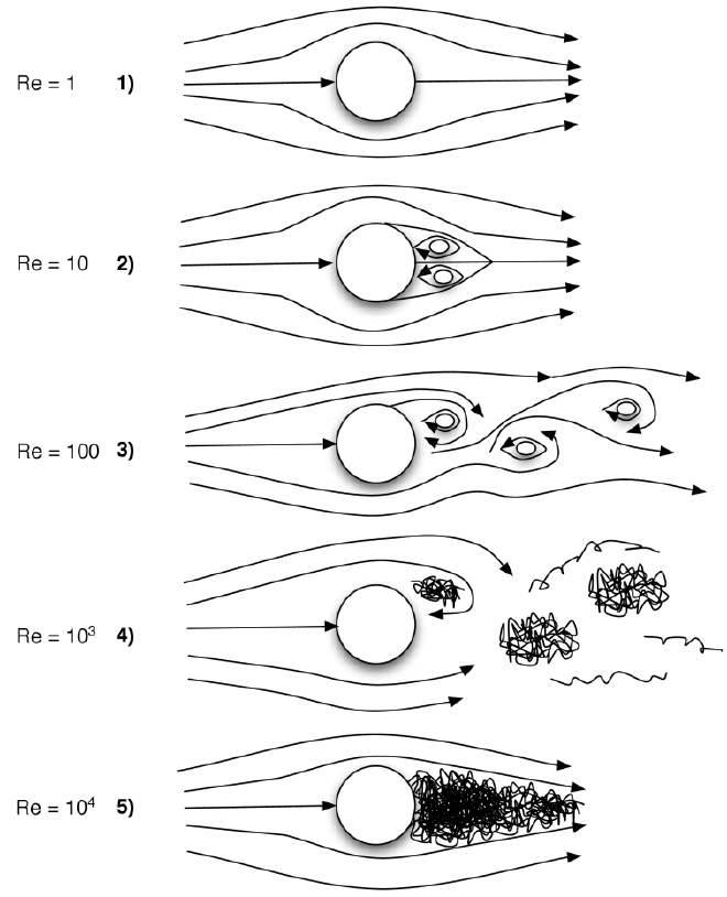
Given its elementary nature, the flow past a circular cylinder is a well-studied case in the field of fluid dynamics. The characteristics of the flow pattern changes with the Reynolds number, resulting in wildly different flow patterns. Representative illustrations of all types of flow behavior are collected in the figure below. Examples of every such flow pattern can be found in van Dyke’s book and on this website. Take for example Figure 24 for attached flow (subfigure 1), Figures 40, 41, 42, 45 and 46 for separated flow with different sizes of separation regions (subfigure 2), Figures 94 and 96 for laminar flow with vortex shedding; von Kármán streets (subfigure 3), Figure 47 for flow shedding turbulent vortices (subfigure 4), and Figure 147 for a fully developed turbulent wake (subfigure 5).
To understand why the nature of the flow changes so drastically with the change in Reynolds number, we must take a look at the governing equations; the Navier-Stokes equations. For an incompressible fluid and with gravitational effects neglected, these read:
$$ \begin{cases} \rho \frac{\partial \mathbf{u}}{\partial t} +\rho (\mathbf{u} \cdot \nabla)\mathbf{u} = \mu \nabla^2 \mathbf{u} - \nabla p \\ \nabla\cdot \mathbf{u} = 0 \end{cases} $$
A derivation of these equations can be found here.
The incompressible Navier-Stokes equation are a set of coupled differential equations that describe the conservation of mass and momentum of a viscous fluid. The dependent fields (i.e., the sought after solution functions) are the vector-valued velocity field \(\mathbf{u}\) and the scalar-valued pressure field \( p\). General forms of the conservation of momentum and mass in partial differential form are: $$ \begin{cases} \frac{\partial}{\partial t}(\rho \mathbf{u} ) + \nabla \cdot ( \rho \mathbf{u} \otimes \mathbf{u} ) = \nabla \cdot \sigma + \rho\mathbf{f} \\ \frac{\partial}{\partial t}\rho + \nabla \cdot ( \rho \mathbf{u} ) = 0 \end{cases} $$ with \( \rho \) the given material density, \(\mathbf{f}\) the specified body acceleration, and \(\mathbf{\sigma}\) the Cauchy stress tensor.
The left-hand-side of the momentum equation can be simplified by expanding the differentiation terms with appropriate chain-rules and by subsequently substituting the mass conservation equation: $$ \frac{\partial}{\partial t}(\rho \mathbf{u} ) + \nabla \cdot ( \rho \mathbf{u} \otimes \mathbf{u} ) = \mathbf{u} \frac{\partial}{\partial t}\rho + \rho \frac{\partial}{\partial t} \mathbf{u} + \mathbf{u} \nabla \cdot ( \rho \mathbf{u} ) + (\rho \mathbf{u}\cdot \nabla )\mathbf{u} \\ = \rho \Big( \frac{\partial}{\partial t}\mathbf{u} + (\mathbf{u}\cdot \nabla )\mathbf{u} \Big) \qquad $$
For an incompressible medium, the density of each moving fluid element remains constant in time. Mathematically, this means that the material derivative of the density is zero: \( \frac{D}{D t}\rho = \frac{\partial}{\partial t}\rho + \nabla \rho \cdot \mathbf{u} = 0 \). This assumption may be used in the earlier mass conservation law to find: $$ \frac{\partial}{\partial t}\rho + \nabla \cdot ( \rho \mathbf{u} ) = \frac{\partial}{\partial t}\rho + \nabla \rho \cdot \mathbf{u} + \rho \nabla \cdot \mathbf{u} = \rho \nabla \cdot \mathbf{u} = 0 $$ Or, in short, \( \nabla\cdot\mathbf{u} = 0 \).
Lastly, a constitutive relation must be substituted in place of the Cauchy stress tensor. First we separate it into its isotropic (\( - p \mathbf{I} \)) and deviatoric (\( \mathbf{\tau}\)) components: $$ \mathbf{\sigma} = \mathbf{\tau} - p \mathbf{I} $$
The incompressible Navier-Stokes equations in their familiar form are then the result of the linear Stokes constitutive relation for the deviatoric stress: $$ \mathbf{\tau} = \mu \Big(\nabla \mathbf{u} + (\nabla\mathbf{u})^T - \frac{2}{3}( \nabla\cdot \mathbf{u})\mathbf{I} \Big) $$ where the last term ensures that \( \mathbf{\tau}\) is deviatoric, but in the case of an incompressible medium it is simply zero. When it may be assumed that the dynamic viscosity \( \mu \) is constant in space, the following holds: $$ \nabla \cdot \mathbf{\tau} = \mu \nabla \cdot \big(\nabla \mathbf{u} + (\nabla \mathbf{u})^T \big) = \mu \nabla \cdot \nabla \mathbf{u} + \mu \nabla (\nabla \cdot \mathbf{u}) = \mu \nabla \cdot \nabla \mathbf{u} = \mu \nabla^2 \mathbf{u} $$ where, again, the divergence-free nature of the velocity field is made use of.
Combining all the above equations results in the incompressible Navier-Stokes equations: $$ \begin{cases} \rho \frac{\partial \mathbf{u}}{\partial t} +\rho (\mathbf{u} \cdot \nabla)\mathbf{u} = \mu \nabla^2 \mathbf{u} - \nabla p + \rho\mathbf{f} \\ \nabla\cdot \mathbf{u} = 0 \end{cases} $$
The first equation represents (in vector form) conservation of linear momentum, and the second equation conservation of mass. While it may seem that there are a multitude of physical parameters that define the solution field (density, viscosity, length and time-scales), there is in effect only a single one: the Reynolds number. This becomes apparent after non-dimensionalizing all quantities in terms of the material parameters (density and viscosity), a characteristic length and a characteristic velocity: \( \hat{L} \) and \( \hat{U} \). Considering each term separately:
- Velocity: \( \mathbf{u} = \hat{U}\, \hat{\mathbf{u}} \)
- Pressure: \( p = \rho \hat{U}^2 \, \hat{p} \)
- Temporal coordinate and time-derivative: \( t = \frac{\hat{L}}{\hat{U}}\, \hat{t} \) so that \( \frac{\partial}{\partial t} = \frac{\hat{U}}{\hat{L}} \frac{\partial}{\partial \hat{t}} \)
- Spatial coordinate and gradient: \( \mathbf{x} = \hat{L}\, \hat{\mathbf{x}} \) so that \( \nabla = \frac{1}{\hat{L}}\, \hat{\nabla} \)
Substitution of these non-dimensionalizations into the earlier Navier-Stokes equations gives the non-dimensionalized Navier-Stokes equations:
$$ \begin{cases} \frac{\partial \hat{\mathbf{u}}}{\partial \hat{t}} + (\hat{\mathbf{u}} \cdot \hat{\nabla})\hat{\mathbf{u}} = \frac{\mu}{\rho \hat{U}\hat{L} } \hat{\nabla}^2 \hat{\mathbf{u}} - \hat{\nabla} \hat{p} \\ \nabla\cdot \hat{\mathbf{u}} = 0 \end{cases} $$
These equations illustrate that (for a domain, initial and boundary conditions fixed in terms of the characteristic quantities) it is really only the Reynolds number \( Re = \frac{\rho \hat{U}\hat{L} }{\mu} \) that defines the solution.
For a small Reynolds number, the viscous term dominates, effectively linearizing the equations (eventually reducing them to the Stokes equations), and for large Reynolds number the viscous term becomes negligible whereby the non-linear inertial term dominates. The transition from small to large Reynolds number thus fundamentally changes the nature of the equations, causing the radical changes of the behavior of the flow illustrated in the earlier figure.
Separation #
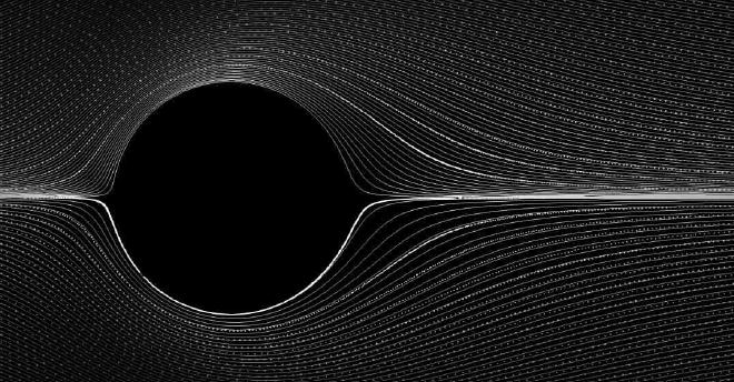
At a sufficiently small Reynolds numbers, in literature typically stated as between 4 and 5, the fluid follows the curvature of the cylinder without separating from its surface. This can be seen in the figure below, which considers the near-limit case of \(Re=4\).
Past this Reynolds number, separation at the rear of the cylinder begins to take place. Then, the boundary layer detaches from the cylinder surface. At the location of the detachment, the “separation point”, the flow velocity is zero, and past that point the fluid particles have reversed their direction. This flow reversal starts to occurs when the negative pressure gradient required to curve the flow around the surface of the cylinder, i.e., the pattern shown in the above figure at \(Re = 4\), becomes too large. Later downstream, the separated flow will reattach at the “reattachment point”, resulting in pockets of circulating fluid (vortices) that are trapped by the surrounding flow. After a Reynolds number of \(Re = 46\) these vortices begin to shed, creating a von Kármán vortex street (see Figure 96 for more detail).
From \(Re = 4\) to \(Re = 46\) the trapped vortex, or separation bubble, grows in length and width. The streamwise length of the separation bubble scales linearly with Reynolds number. The Reynolds number dependency of the location of the separation point, characterized by the “separation angle” as the angle along the cylinder surface, is somewhat more elusive. It has been studied extensively, both experimentally and numerically, as can be seen in the following figure:
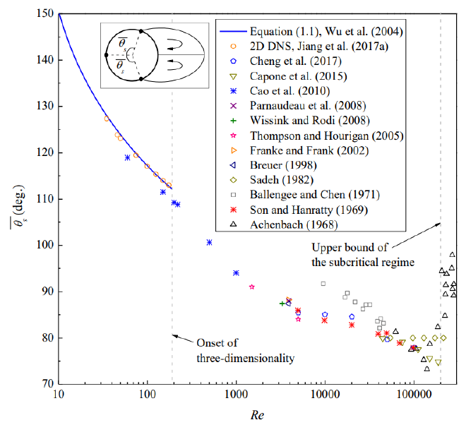
Fitting the data provides an empirical relationship between the separation angle and Reynolds number, as described by the following formula: $$ \theta_S = 95.7 + 267.1Re^{-\frac{1}{2}} - 625.9Re^{-1} +1046.6Re^{\frac{-3}{2}} $$ The current figure, Figure 42, involves a Reynolds number of \(26\). This formula then predicts a separation angle equal to \(132\) degrees, corresponding well with the experiment and the simulation.
Simulation #
The CFD simulation program used to perform the above simulations is Simcenter StarCCM+. The two-dimensional nature of the flow permits the use of 2D flow models to decrease the computational time.
Boundary conditions and computational domain #
With the Reynolds number (\(Re=26\)) given in the caption of the original figure the entire flow field is determined in terms of non-dimensionalized quantities. StarCCM+ requires dimensionalized quantities, however. The caption also indicates that the photograph is made by Sadathoshi Taneda, who provided multiple pictures from the original book. In other pictures, Mr. Taneda uses a cylinder with a diameter of \(1 \)cm, and it seems to be the case that he uses the same experimental setup for all photographs. With the length dimension and the material parameters determined, the velocity can be calculated: \(Re = \frac{\rho u D}{\mu}\), or \( u = \frac{\mu \, Re}{\rho \, D} = 2.6 \)mm/s. Based on these quantities, the computational domain and boundary conditions are defined, as illustrated in the figure below.
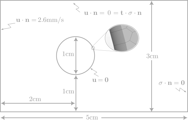
The total domain has a length of \(5 \)cm and the distance from the centre of the cylinder to the end of the domain is \(3 \)cm, leaving \(2 \)cm in front of the circle centre. The height of the domain is \(3 \)cm, with the centre of the cylinder at \(1.5 \)cm. The total domain of the Figure was not given in the caption but derived from the original figure. To avoid too disruptive wall-influences from the top and bottom wall, these are set as symmetry planes. The cylinder is set as a wall with a no-slip boundary condition applied to it. The inflow is set as a velocity inlet with a velocity of \(2.6\)mm/s in the normal direction and the outlet is set as a no-traction outlet.
Meshing #
The mesh created for this simulation is based on a quadrilateral 2D mesh, which is one of many meshing options from STARCCM+. After selecting the quadrilateral 2D mesh, the polygonal mesh option is used. This mesh consists of polyhedral-shaped cells. In comparison to an equivalent tetrahedral mesh, a polygonal mesh contains five times fewer cells and is documented to be more accurate, more stable and less diffusive. The base size of the mesh is set to \(0.02 \)m and the growth rate to 1.004. As the near-boundary behavior of the flow is of crucial importance for accurate prediction of flow separation, a highly refined prism boundary layer mesh is created. A total amount of 34386 cells were created. Some representations of the mesh can be found below.
Fluid model #
The simulation was run with a laminar, steady model with water as the flowing fluid. For the simulation, a total of 3500 iterations were simulated, of which the velocity data was exported to an Ensight Gold case file, so it could be processed in Paraview. All models used in STARCCM+ and the STARCCM+ result for Figure 40 after 3500 iterations are shown below.
Visualization #
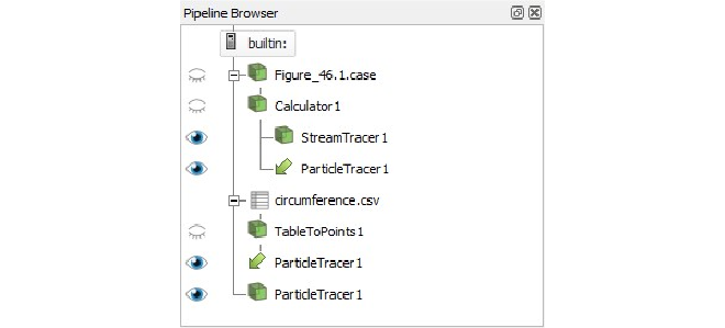
Paraview is used for the post-processing and visualization of the simulation. After importing the velocity data, a calculator filter is used to compute the velocity vector from the exported x-velocity and y-velocity data. Next, the circumference of the cylinder is covered in particles with the code supplied at the bottom of this page. In combination with a TableToPoints filter, this is used as an input seed for the Particletracer filter. The Particletracer filter together with the Streamtracer filter is used to produce the final visualization shown at the start of this web post. The complete pipeline looks as follows:
And the code used for creating the particles at the circumference of the cylinder can be found below.
n = 720;

angles = linspace(0, 2*pi, n);
radius = 0.00501;
xCenter = 0;
yCenter = 0;
X = -radius * cos(angles) + xCenter;
Y = -radius * sin(angles) + yCenter;

P = zeros(n+1,3);
P(1,:) = [1,2,3];
P(2:end,1) = X;
P(2:end,2) = Y;

writematrix(P,'circumference.csv')