Fig 37. Global separation over an inclined plate
Table of Content
Air bubbles in water show the turbulent flow field around an inclined plate at Reynolds number \(Re = 10000\). At 20\(^{\circ}\) inclination relative to the oncoming flow, the flow fully separates from the entire upper surface of the plate and creates a turbulent wake. The turbulent boundary layer is of highly chaotic and unsteady nature. For comparison, a transient simulation was created in Simcenter StarCCM+ using the SST turbulence model. Photograph by ONERA photograph, Werlé 1974
Turbulence transition #
Turbulent flow is characterized by its chaotic and irregular behaviour. Although turbulent flow is often encountered and widely relevant to engineers, accurately modelling and predicting it has been the subject of intense scientific research over the past few decades. In contrast to the predictable and easy to model laminar flow, turbulent flow requires complex models to solve the million dollar Navier-Stokes equations. $$ \rho (\frac{\partial\textbf{u}}{\partial t} + \textbf{u}\cdot \nabla \textbf{u}) = -\nabla p + \nabla \cdot (\mu (\nabla \textbf{u} + (\nabla \textbf{u}^T))-\frac{2}{3}\mu(\nabla \cdot \textbf{u})\textbf{I}) + \textbf{F} $$ Numerically solving the Navier-Stokes equations is extremely computationally expensive because of the largely different mixing-length scales present in turbulent flow. From modelling planet sized meteorological effects such as rotating tropical cyclones to modelling microscopic effects of vortex energy dissipation due to viscous losses, the Navier-Stokes equations need to be adjusted for numerical computations.
More in-depth information on modelling turbulence using the so-called Reynolds-averaged Navier-Stokes equations (RANS) can be found on Fig. 47. Details about deriving different types of turbulence models, such as k-epsilon, k-omega and SST, is also explained there. As was done in the posts for Fig. 35, Fig. 36 and Fig. 47, this post serves as a comparison and evaluation of different turbulence models for different simulations setups of the equivalent experiment setup from the original figures in the book.
Simulation #
All of the simulations of the inclined plate experiment were carried out in Simcenter StarCCM+ using the k-epsilon, k-omega and SST turbulence models. The differences in results of each of the turbulence models will be discussed in the ‘Visualization’ section of this post, since the differences become apparent during post-processing.
Computational domain #
Considering the information about the experiment setup given in the caption of Figure 37 and the experiment being very similar to the two previous pictures, the computational domain, boundary conditions and finite volume mesh can be set up. The visualization of the flow field in this experiment is done with air bubbles in water. Knowing that the characteristic Reynolds number is \(Re = 10000\) based on the length of the plate, the length can be calculated to be \(0.1\ m\) and the inlet velocity \(0.1\ m/s\). As for the two previous posts, this experiment closely resembles that of flow over an airfoil, with the angle of attack increased to \(20^{\circ}\) for this experiment. The plate geometry was kept the same, with beveled edges and \(2\)% thickness.
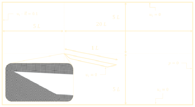
The domain size is given in the figure above. The base size of the quadrilateral FVM mesh is set to \(0.001\ m.\) To save on computational expenses, this base size is only applied in the region near the inclined plate. The custom mesh controls available in StarCCM+ are used to coarsen the mesh in the far-field parts of the domain. The domain walls have an element size of \(0.3\ m\) (\(30000\)% of base size) and the global growth rate is set to \(1.1\). Further refinement is added on both the leading and trailing edge of the plate, where separation is expected to occur. In this area, the mesh is refined to \(25\)% of the base size. The turbulent separation region shown in the original figure also has \(50\)% refinement applied to it, while the wall boundary and near wall region is refined with an inflation layer. This layer consists of \(24\) prism layers with a stretch factor of \(1.2\) and a total thickness of \(0.002\ m\) (\(200\)% of base size). The total cell count is \(75077\) and some figures of this mesh and the refinement region can be seen below.
StarCCM+ setup #
The simulation setup in StarCCM+ is generally the same as for the two other inclined plate simulations and are already referenced above. The simulation is run a total of three times, using the low Reynolds number k-epsilon model, one using Wilcox’s (2008) k-omega model and a last one using Menter’s SST model. These simulations are run in a transient environment in order to capture the instantaneous flow field and turbulence.
Visualization #
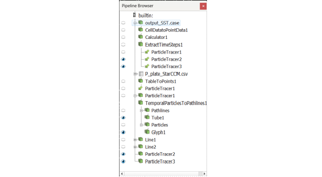
The visualization setup for Paraview is very similar to the one mentioned in the post for Fig. 47 about flow around a circular cylinder and more details can be found there. Since a highly chaotic and turbulent flow field is expected, random particle injection and particle tracing is used to visualize the velocity field of the simulation results. The ParaView pipeline used for this visualization can be seen below.
Turbulence model comparison #
Accurately comparing the simulation results of the different turbulence models to the actual experiment and between each other is hard to do because of the highly chaotic and turbulent nature of the instantaneous flow field captured in the original picture. Having considered this, the SST turbulence model seems to give the most accurate representation of the flow field, at least in terms or correctly predicting the relevant length scales. This comparison can be seen in the slider figure at the very top of the page. As for the visualization results provided by the k-epsilon and k-omega turbulence models, these are shown below and can be compared using the slider.
From the comparisons above, the expected behaviours of the different turbulence models are observed. As explained in the posts about flow over a low angle inclined plate ( Fig. 35 and Fig. 36) and considering the turbulence model derivations explained in the post for Fig. 47, the k-epsilon shows a clear lack of near-wall turbulence prediction. On the other hand, the k-omega predicts a higher amount of eddies forming both on the top side of the plate as well as in the wake of the plate. Comparing this to the results of the SST simulation and the real experiment picture, these do not seem to show any vorticity in the wake of the plate. Although the SST model predictions best match those of the actual experiment picture, the small scale turbulence and chaos is not really captured. The SST model only seems to depict large scale eddies. Although the k-omega model predicts a larger amount of largely differing eddy sizes, there is a still clear presence of recurring large scale eddies, as can be seen halfway down the length of the plate and in the wake of the inclined plate.
In all three cases, this simulation setup starts showing the general limitations of Reynolds-averaged Navier-Stokes (RANS) models. As the name suggests, these models are based on the average velocities of the flow field. More information about the derivation of the RANS equations can be found in the theory section of this post. Because RANS models aim to model turbulent phenomena on the mean velocity scale, they struggle to show small scale chaos and turbulence that would be expected in any instantaneous flow field. Also, because of their average velocity nature, RANS models are better suited for steady state simulations of high Reynolds number flows, where small fluctuations in the velocity field are not of high importance.
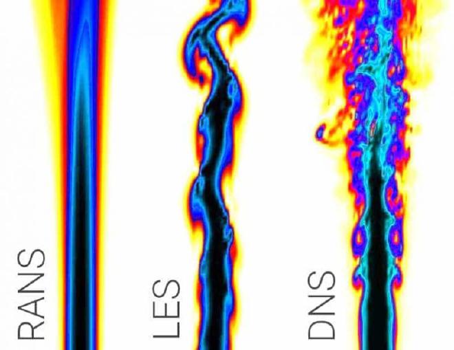
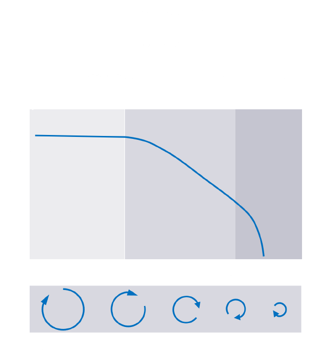
To better understand the limitation of RANS models for the simulations shown above, the figure below gives a representation of where RANS models are situated on the eddy scale spectrum compared to other types of numerical simulation approaches.
This figure mentions DNS, which stands for Direct Numerical Simulation. This is in fact not a turbulence model, rather a direct simulation of the Navier-Stokes equations at the entire temporal and spatial turbulence scales. While resolving the Navier-Stokes equations numerically still requires a computational grid, it is extremely fine and makes this method massively computationally expensive, which is simply not a viable simulation method for most cases. DNS is reserved for very small computational domains and trivial flow situations, but is accurate enough to serve as validation data for CFD models.
Next, this figure mentions LES models, which stands for Large Eddy simulation. These models also fully resolve the Navier-Stokes equations, however only down to a certain scale. Below this scale, a type of low-pass filter is applied to the Navier-Stokes equations, which spatially and temporally averages them. This greatly saves on computation costs while still providing highly accurate results.
LES models still have very high computation costs compared to RANS models, which model the entire eddy size spectrum. The low computational costs are what make RANS models so popular. However, there is one more popular type of turbulence model, namely DES models. DES stands for Detached Eddy Simulation. These models can be considered hybrids between RANS models ans LES models.
The figure below ( link ) shows the difference in instantaneous flow field results between the above mentioned types of numerical simulation approaches.