Fig 36. Leading-edge separation on a plate with turbulent reattachment
Table of Content
Air bubbles in water show the turbulent flow field and turbulent reattachment on an inclined plate at Reynolds number \(Re = 50000\). At 2.5\(^{\circ}\) inclination relative to the oncoming flow, the flow separates from the upper surface, creating a turbulent boundary layer at the leading edge before reattaching to the inclined plate. The separation region creates a recirculating turbulent boundary layer. For comparison, a transient simulation was created in Simcenter StarCCM+ using the SST turbulence model. Photograph by ONERA photograph, Werlé 1974
Turbulence transition #
In general, this experiment and simulation setup is the same as described in this post, except that the characteristic Reynolds number is increased by a factor of 5. Practically speaking this means that the inlet velocity is increased by a factor of 5, while all other parameters remain the same. With the Reynolds number being the ratio between inertial and viscous forces, higher Reynolds number flows tend to display higher turbulence and chaos in the flow field, which is what can be observed in this experiment picture. As for the recirculating boundary layer at the leading edge of the plate, it is much less visible than in the picture of the same experiment at Reynolds number \(Re = 10000\). However, the streamlines of this flow field, visualized with the air bubbles in the water and the shutter speed of the camera, clearly show a recirculating bubble as a boundary layer at the leading edge.
Simulation #
All of the simulations of the inclined plate experiment were carried out in Simcenter StarCCM+ using the k-epsilon, k-omega and SST turbulence models. Since this simulation setup closely resembles that of this post, more detailed information about the computational domain and finite volume mesh setup can be found there. This post will focus mainly on the differences in results of each of the turbulence models and will be discussed in the ‘Visualization’ section of this post. More details and information about RANS turbulence models, can be found in this post.
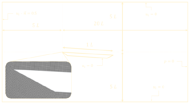
Computational domain #
As mentioned above, the experiment setup for this picture, and thus the simulation setup are identical to the one mentioned in the previous post about a \(2.5^{\circ}\) inclined plate with the only change in the simulation setup being the increase from \(0.1\ m/s\) to \(0.5\ m/s\) for the inlet velocity boundary condition. This changes the characteristic Reynolds number from \(Re = 10000\) to \(Re = 50000\) as is the case for this experiment setup. For visualization purposes, the computational domain is shown again below.
StarCCM+ setup #
The simulation setup in StarCCM+ is the exact same as mentioned in this post about flow over a circular cylinder. More details and information about the simulation setup can be found there. What’s important to note is that three simulations were run in a transient environment, one using the low Reynolds number k-epsilon model, one using Wilcox’s (2008) k-omega model and a last one using Menter’s SST model.
Visualization #
Again, the detailed steps to obtaining the final visualizations of this simulation setup in
Paraview can be found in the previous post. The main visualization feature is the StreamTracer filter, since away from the turbulent boundary layer, the air bubbles in the water mainly show the streamline of this flow field. All of the visualizations are taken at the same time step with respect to the most accurate visualization compared to the original picture, which again is the SST model simulation. All of the visualizations can be seen in the slider figures below and the comparison between the SST model and the actual experiment picture can be seen at the very top of the page.
Looking at the comparison between the visualization of the SST model and the original experiment figure at the top of the page, it becomes apparent that the small scale turbulent phenomena is not really captured. Although the boundary layer height of the recirculating bubble seems to be accurately predicted, the actual turbulence and chaos of the turbulent boundary layer is not really displayed. Comparing the visualization of the k-omega and SST model, the boundary layer height prediction is almost identical, but the SST model seems to depict slightly more turbulence along the top and the wake of the plate. However, when looking at the k-epsilon model visualization, the recirculating boundary layer at the leading edge seems to be completely missing. A likely explanation for this is that the low Reynolds number k-epsilon model is not well suited for this simulation. A deeper analysis of this will be given in the next section.
Turbulence model comparison #
To give a more quantitative comparison and evaluation between the different turbulence models, the boundary layer height in the recirculating bubble can be measured. This is done the same way as described in the ‘Turbulence model comparison’ section of this post. The slider figures below show the boundary layer height \(\delta\) for different boundary layer definitions. Namely $$ u(x, \delta) = a \cdot u_{\infty} $$ with \(a\) the percentage of the freestream velocity \(u_{\infty}\) (\( = 0.5\ m/s\) in this case) between \(50\)% and \(95\)%.
As can be seen in the slider figures above, the k-omega and SST model show very similar results for the boundary layer height over the first \(15\)% of the plate length. After this, the SST model seems to predict a flatter boundary layer profile. Since the simulation results can only be compared to the picture of the experiment and not to actual experimental data, it is difficult to say which model is the most accurate, especially since the simulation visualizations do not match the actual picture that well. However, the simulations for flow around a cylinder at \(Re = 2000\) and for flow around a \(2.5^{\circ}\) inclined plate at \(Re = 10000\) have shown that the SST model consistently provides the best visual results between the three RANS models tested for these simulations. It is still interesting to highlight the differences between the models, even without reference data.
However, comparing the k-epsilon model to the SST model reveals a large discrepancy between the two. As could already be seen in the visualizations above, the k-epsilon model shows a very unexpected boundary layer shape. Although the boundary layer height \(\delta_{95}\) (at \(95\)% of the freestream velocity) doesn’t seem that far off the results of the SST model, the height prediction of other velocities are largely different.
One of the hypotheses for these seemingly faulty results of the k-epsilon model is that the low Reynolds number formulation of this model was used. This means that compared to the standard k-epsilon model, empirical damping functions (\(f_1\), \(f_2\), \(f{\mu}\)) are applied to the coefficients \(C_{1\epsilon}\) and \(C_{2\epsilon}\) $$ \begin{align*} \frac{\partial \rho k}{\partial t} + \frac{\partial \rho k u_i}{\partial x_i} &= \frac{\partial}{\partial x_j} \left( \frac{\mu_t}{\sigma_k} \frac{\partial k}{\partial x_j} \right) + P_k - \rho \epsilon \\ \frac{\partial \rho \epsilon}{\partial t} + \frac{\partial \rho \epsilon u_i}{\partial x_i} &= \frac{\partial}{\partial x_j} \left( \frac{\mu_t}{\sigma_{\epsilon}} \frac{\partial \epsilon}{\partial x_j} \right) + f_1 C_{1\epsilon} \frac{\epsilon}{k} P_k - f_2 C_{2\epsilon} \frac{\rho \epsilon^2}{k} \end{align*} $$ and the eddy viscosity \(\mu_t\) also adjusted with $$ \mu_t = f_{\mu} C_{\mu} \frac{k^2}{\epsilon} $$ However, the general guideline for this low Reynolds number k-epsilon is that it should only be used for \(y^+\) values below 30, with \(y^+\) known as the dimensionless wall distance. This value can be interpreted as a local Reynolds number for near wall turbulence and states that velocity distributions in the near-wall region are very similar for almost all turbulent flows. This is also known as the universal law of the wall [1]. For \(y^+\) values below 30, the mesh inflation layer on wall boundaries also plays a large role for accurate simulation results. Unfortunately, these parameters were not considered when setting up this simulation and the low Reynolds number k-epsilon model was chosen, just as it was used for the \(Re = 10000\) inclined plate simulation. Also, as mentioned above, the same mesh settings were used for both of these simulations.
One further metric that can be compared between the different turbulence model results (although the k-epsilon model shouldn’t necessarily be considered because of the outlying results) is the lift coefficient produced by the inclined plate. For this, a report monitor was set up in StarCCM+ and the data was exported at each timestep. To properly visualize the data, the following MATLAB script was used, with the resulting plot shown below.
kepsilon    = readtable("Cl data\HighReInclinedPlate_Cl_data_kepsilon.csv");
iters1      = kepsilon.Iteration;
t1          = iters1/(20000/15);
cl_kepsilon = kepsilon.ClMonitor_ClMonitor;

komega      = readtable("Cl data\HighReInclinedPlate_Cl_data_komega.csv");
iters2      = komega.Iteration;
t2          = iters2/(20000/15);
cl_komega   = komega.ClMonitor_ClMonitor;

sst         = readtable('Cl data\HighReInclinedPlate_Cl_data_SST.csv');
iters3      = sst.Iteration;
t3          = iters3/(20000/15);
cl_sst      = sst.ClMonitor_ClMonitor;

figure(1)
hold on
plot(t1,cl_kepsilon)
plot(t2,cl_komega)
plot(t3,cl_sst)
hold off
xlim([0 15])
ylim([0.15 0.3])
grid on
grid minor
title('Lift coefficient using different turbulence models')
xlabel('Physical time [s]')
ylabel('Lift coefficient [-]')
legend('k-epsilon','k-omega','SST')
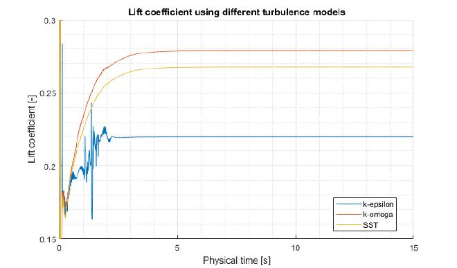
As can be seen from the graph, the k-epsilon results can definitely be considered to be outliers. However, it is interesting to note the slight difference of about \(3.5\)% between the steady-sate lift coefficient of the SST model and that of the k-omega model. This graph also shows that the SST model and k-omega model show an almost identical time at which steady-state is reached.