Fig 94. Kármán vortex street behind a circular cylinder at R=140

Experiment

Simulation

“Water is flowing at 1.4 cm/s past a cylinder of diameter 1cm. Integrated streamlines are shown by electrolytic precipitation of white colloidal smoke, illuminated by a sheet of light. The vortex street is seen to grow in width downstream for some diameters.” Photograph by Sadathoshi Taneda

Theory #

This post is part of a series on flow separation, studied for the case of flow past a circular cylinder at different Reynolds numbers. The full series is:

• Figure 24: Circular cylinder at R=1.54.
• Figure 40: Circular cylinder at R=9.6.
• Figure 41: Circular cylinder at R=13.1.
• Figure 42: Circular cylinder at R=26.
• Figure 45: Circular cylinder at R=28.4.
• Figure 46: Circular cylinder at R=41.
• Figure 96: Kármán vortex street behind a circular cylinder at R=105.
• Figure 94: Kármán vortex street behind a circular cylinder at R=140.

An overview of these posts can be viewed here:

Laminar, unsteady flow #

When the Reynolds number of the flow past the circular cylinder exceeds the “critical Reynolds number”, which is roughly \(Re=46 \), the trapped vortices shown in the earlier figures of this series detach from the cylinder and are advected with the flow. This behavior is oscillatory; shedding occurs successively from the top and bottom of the cylinder. The resulting flow pattern is called a “von Kármán vortex street”. Despite its unsteady nature, the flow is still laminar; the advected vortices of layers of fluid circulating around each other, as is nicely shown in Figure 98. The vortices become turbulent when the Reynolds number exceeds roughly \(Re=189 \), see e.g. Figure 47.

Hopf Bifurcation #

The point at which a system switches from a stable stationary state to a stable oscillatory state is called a Hopf Bifurcation. It is a fixed critical point in a system where the system loses its primary stability. Indeed, for flow behind a circular cylinder, the first Hopf bifurcation arises when the Reynolds number reaches its critical point, \(Re = 46\), and a second bifurcation point can be identified at a Reynolds number of approximately \(Re = 189\). This second Bifurcation point marks the onset of turbulent motions, and with increasing Reynolds number the flow patterns disappear into a chaotic flow.

Strouhal number #

The periodic nature of the flow that arises after a Reynolds number of \(46\) can be characterized with a dimensionless number, the Strouhal Number. The Strouhal number is defined as follows:

$$ St = \frac{f\,\hat{L}}{\hat{U}} $$

where \(f\) is the frequency of vortex shedding, \(\hat{L}\) is a characteristic length scale (e.g. the diameter of the cylinder) and \(\hat{U}\) is a characteristic velocity.

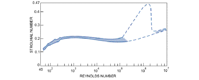
The Strouhal number has a dependency on the Reynolds number but is for a large Reynolds number interval (\(250 < Re < 2 \cdot 10^5\)) approximately constant and equal to \(0.2\) as can be seen in the figure below.

Simulation #

The CFD simulation program used to perform the above simulations is Simcenter StarCCM+.

Boundary conditions and computational domain #

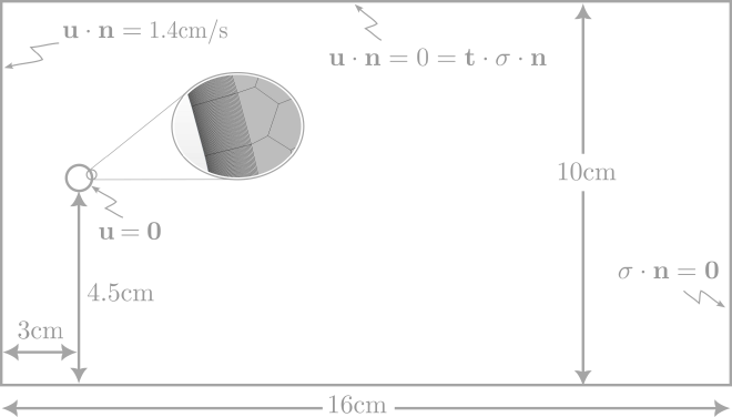
The velocity (\(u = 1.4 cm/s = 1.4 \))cm/s and cylinder diameter (\(D = 1 \))cm are given in the caption of the figure. The domain size of the experiment itself is not given in the caption, so reasonable estimates need to be made. The choices made for the computational domain and boundary conditions can be seen in the figure below. The total domain has a length of \(19\)cm to accommodate a number of travelling vortices. The distance fro the center of the cylinder to the end of the domain is \(16 \)cm, leaving \(3 \)cm in front of the center. The height of the domain is \(10 \)cm, with the center of the cylinder at \(5 cm\). To avoid major influences of the top and bottom boundary on the flow around the vortex street, the top and bottom of the domain are set as symmetry planes. The cylinder is set as a wall with a no-slip boundary condition applied to it. The inflow is set as a velocity inlet with a velocity of \(1.4\)cm/s, and the outlet is set as a no-traction outlet.

Meshing #

The mesh is created in the same fashion as described in Figure 42. For this larger domain, this results in a mesh with a total amount of 135212 cells. Some representations of the mesh can be found below.

Fluid model #

The simulation was run with a laminar, unsteady model with water as the flowing fluid. For the simulation, a second-order implicit unsteady solver with a time-step of \(0.025 sec\) was used. A total of 1400 time steps were run with 50 iterations per time step, resulting in 70000 iterations and a physical time of 35 sec. The velocity data of all time steps was exported to an Ensight Gold case file, so it could be processed in Paraview. All models used in STARCCM+ and the STARCCM+ result after 1400 time steps can be found below.

Visualization #

Details of the visualization procedure may be found in the post of Figure 42.